Note
Go to the end to download the full example code
ElGohary Turning Algo#
Warning
The ElGohary turning algorithm could not be properly validated as part of the Mobilise-D project, as no clear consensus exists what a “turn” is. This makes it difficult to design a suitable reference system, which nature of calculating turns does not bias the results fundamentally.
This example shows how to use the ElGohary turning algorithm. It uses the angular velocity around the SI axis of a lower back IMU to detect turns.
Loading data#
Note
More infos about data loading can be found in the data loading example.
We load example data from the lab dataset together with the Stereophoto reference system. We will use the Stereophoto output for turns (“td”) as ground truth, as it is the most accurate reference system available in the dataset. Still, the turn detection might not be fully reliable. Note, that the INDIP system, also uses just a single lower back IMU to calculate the turns. Hence, it can not really be considered a reference system, in this context.
The turn algorithm requires the data to be in the body frame (see the User Guide on this topic).
We use the to_body_frame function to transform the data, as we know that the sensor was well aligned, with the
expected sensor frame conventions.
from mobgap.data import LabExampleDataset
from mobgap.utils.conversions import to_body_frame

example_data = LabExampleDataset(
    reference_system="Stereophoto", reference_para_level="wb"
)

single_test = example_data.get_subset(
    cohort="HA", participant_id="001", test="Test11", trial="Trial1"
)
imu_data = to_body_frame(single_test.data_ss)
reference_wbs = single_test.reference_parameters_.wb_list

sampling_rate_hz = single_test.sampling_rate_hz
Note, that the reference turns don’t use the 45 deg lower cutoff for turns by default. Hence, we apply this here for consistency.
ref_turns = single_test.reference_parameters_.turn_parameters.query(
    "angle_deg.abs() >= 45"
)
Applying the algorithm#
In a typical pipeline, we first identify the gait sequences and then apply the turning detection algorithm to each gait sequence individually. However, the turning algorithm can also be applied to the whole recording at once. Though, it might produce false positives, in “non-walking” segments.
Below we show both approaches, starting with the whole recording. This allows us to visualize how the algorithm works.
from mobgap.turning import TdElGohary

turning_detector = TdElGohary()

turning_detector.detect(imu_data, sampling_rate_hz=sampling_rate_hz)
turn_list = turning_detector.turn_list_
turn_list
We can also extract additional debug information from the algorithm.
The yaw-angle gives us the estimated orientation of the lower back in the axis of the turning.
The raw_turn_list_ gives us the raw detected turns, before filtering them based on duration and angle.
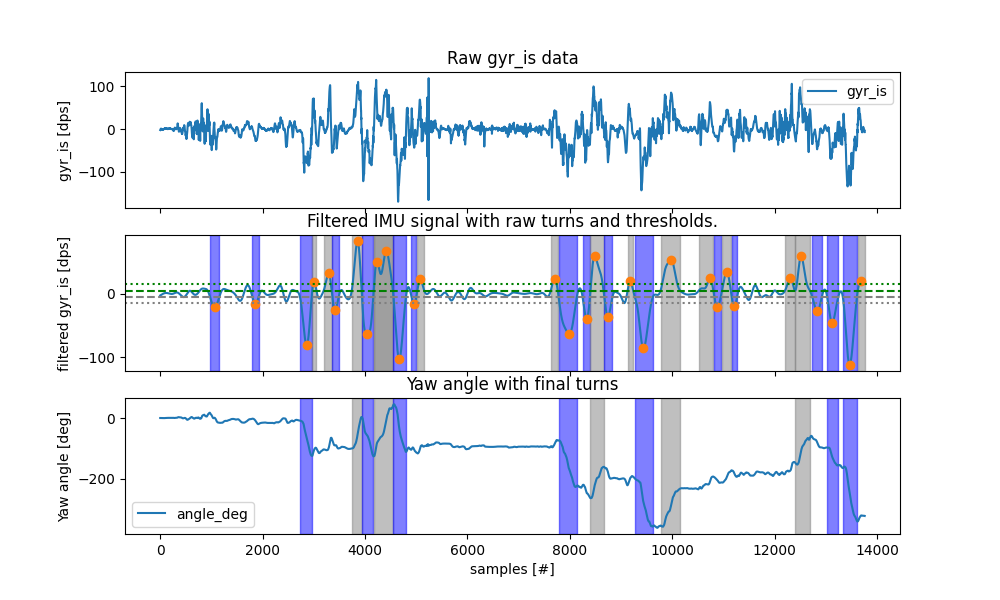
To better understand, how things work, we can plot all the results together.
We can see that after filtering the signal, the algorithm identifies peaks in the signal that are higher in absolute
values than the min_peak_angle_velocity_dps (dotted lines).
Around these “turn-centers” the turn is defined as the region until the signal drops below the
lower_threshold_velocity_dps (dashed lines).
We then look at the duration and the angle of the detected turns and filter them based on the provided thresholds.
We can see that at the end, only a small number of turns remain.
Most of the raw turns are filtered out by the allowed_turn_angle_deg threshold, which is set to 45 degrees.
import matplotlib.pyplot as plt


def plot_turns(algo_with_results: TdElGohary):
    fig, axs = plt.subplots(3, 1, figsize=(10, 6), sharex=True)
    axs[0].set_ylabel("gyr_is [dps]")
    if algo_with_results.global_frame_data_ is None:
        data = algo_with_results.data
        axs[0].set_title("Raw gyr_is data")
        axis = "gyr_is"
    else:
        data = algo_with_results.global_frame_data_
        axs[0].set_title("Raw gyr_is data (global frame)")
        axis = "gyr_gis"
    data.reset_index(drop=True).plot(y=axis, ax=axs[0])

    axs[1].set_title("Filtered IMU signal with raw turns and thresholds.")
    axs[1].set_ylabel("filtered gyr_is [dps]")
    filtered_data = (
        algo_with_results.smoothing_filter.clone()
        .filter(data[axis], sampling_rate_hz=sampling_rate_hz)
        .filtered_data_
    )
    filtered_data.reset_index(drop=True).plot(ax=axs[1])

    raw_turn_list = algo_with_results.raw_turn_list_
    # Plot turn centeres
    axs[1].plot(
        raw_turn_list["center"],
        filtered_data.iloc[raw_turn_list["center"]],
        "o",
    )
    # Plot start and end of turns as regions
    for i, row in raw_turn_list.iterrows():
        axs[1].axvspan(
            row["start"],
            row["end"],
            alpha=0.5,
            color="gray" if row["direction"] == "left" else "blue",
        )

    # Draw dashed line at +/- velocity_dps
    axs[1].axhline(
        algo_with_results.lower_threshold_velocity_dps,
        color="green",
        linestyle="--",
        label="velocity_dps",
    )
    axs[1].axhline(
        -algo_with_results.lower_threshold_velocity_dps,
        color="gray",
        linestyle="--",
    )

    # Draw dottet line at +/- height
    axs[1].axhline(
        algo_with_results.min_peak_angle_velocity_dps,
        color="green",
        linestyle=":",
        label="height",
    )
    axs[1].axhline(
        -algo_with_results.min_peak_angle_velocity_dps,
        color="gray",
        linestyle=":",
    )

    axs[2].set_title("Yaw angle with final turns")
    axs[2].set_ylabel("Yaw angle [deg]")
    axs[2].set_xlabel("samples [#]")
    algo_with_results.yaw_angle_.reset_index(drop=True).plot(ax=axs[2])

    # Plot start and end of turns as regions
    for i, row in algo_with_results.turn_list_.iterrows():
        axs[2].axvspan(
            row["start"],
            row["end"],
            alpha=0.5,
            color="gray" if row["direction"] == "left" else "blue",
        )

    fig.show()


plot_turns(turning_detector)
Now that we understand how the algorithm works, we apply it in the context of a typical pipeline using the
GsIterator in combination with the reference WBs.
This allows us to compare the results to the reference system.
from mobgap.pipeline import GsIterator

iterator = GsIterator()

for (gs, data), result in iterator.iterate(imu_data, reference_wbs):
    td = turning_detector.clone().detect(
        data, sampling_rate_hz=sampling_rate_hz
    )
    result.turn_list = td.turn_list_

turns = iterator.results_.turn_list
turns
We can compare this to the reference turns.
The results look reasonable, but we can see that in gs 3 and 5 the algorithm was not able to detect the smaller turns with lower turning angles.
Working in the global coordinate system#
The original ElGohary paper uses on-board sensor fusion to track the orientation of the sensor. This information is used to transform all sensor data into the global coordinate system. This should make the identification of the inferior-superior (IS) axis more robust.
We did not use this approach within Mobilise-D, to avoid introducing an additional source of error through a sensor fusion algorithm. However, the result of the algorithms can be significantly influenced by that decision, in particular if participants have a lot of body sway of walk bend forward. Below we show two approached on how you could use the algorithm with a global frame estimation.
1. Using the internal global frame estimation#
For this we pass an instance of the MadgwickAHRS algorithm to estimate the global orientation of the sensor to the algorithm.
from mobgap.orientation_estimation import MadgwickAHRS

orientation_estimator = MadgwickAHRS()
Now we can apply the algorithm again. We are going to apply it to the entire recording to show the step-by-step process.
turning_detector_global = TdElGohary(
    orientation_estimation=orientation_estimator
)

turning_detector_global.detect(imu_data, sampling_rate_hz=sampling_rate_hz)
plot_turns(turning_detector_global)
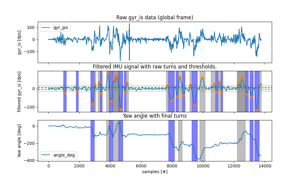
Based on the plotted results, we can see that the algorithm identifies basically the same turns as before.
The same can be observed, when applying the algorithm per GS. The turns are almost identical as before, indicating, that the global frame transformation was not really required for this specific dataset.
iterator = GsIterator()

for (gs, data), result in iterator.iterate(imu_data, reference_wbs):
    td = turning_detector.clone().detect(
        data, sampling_rate_hz=sampling_rate_hz
    )
    result.turn_list = td.turn_list_

turns_global_per_gs = iterator.results_.turn_list
turns_global_per_gs
Alternatively, we could also use the global frame estimation to transform the data into the global frame before applying the algorithm.
2. Transforming the data into the global frame#
For this, we first estimate the global frame for the entire recording and then put the rotated data into the Gait Sequence Iterator. Theoretically, this should yield slightly better results, as the Madgwick algorithm always needs a certain amount of time to converge to the correct orientation. By running it once over the entire data, these convergence period should only happen once at the beginning of the entire recording and not affect the start of each gait sequence.
ori_estimator = orientation_estimator.clone().estimate(
    imu_data, sampling_rate_hz=sampling_rate_hz
)
imu_data_global = ori_estimator.rotated_data_

iterator = GsIterator()

for (gs, data), result in iterator.iterate(imu_data_global, reference_wbs):
    td = turning_detector.clone().detect(
        data, sampling_rate_hz=sampling_rate_hz
    )
    result.turn_list = td.turn_list_

turns_global = iterator.results_.turn_list
turns_global
Which of the two approaches is better, depends on multiple factors. If the global frame should be used generally, further investigation is needed.
Total running time of the script: (0 minutes 3.557 seconds)
Estimated memory usage: 13 MB