Note
Go to the end to download the full example code
GSD Paraschiv-Ionescu#
This example shows how to use the two variants of the Gait Sequence Detection (GSD) algorithm by
Paraschiv-Ionescu et al.
The normal version called GsdIonescu uses a fixed signal activity threshold and a simplified filter chain and the
adaptive version called GsdAdaptiveIonescu, uses an “automatic” threshold calculation and a more complex filter
chain.
We start by defining some helpers for plotting and loading the data. You can skip them for now and jump directly to “Performance on a single lab trial”, if you just want to see how to apply the algorithm.
# Plotting Helper
# ---------------
# We define a helper function to plot the results of the algorithm.
# Just ignore this function for now.
import json

import matplotlib.pyplot as plt
import pandas as pd
from mobgap import PACKAGE_ROOT


def plot_gsd_outputs(data, **kwargs):
    fig, ax = plt.subplots()

    ax.plot(data["acc_x"].to_numpy(), label="acc_x")

    color_cycle = iter(plt.rcParams["axes.prop_cycle"])

    y_max = 1.1
    plot_props = [
        {
            "data": v,
            "label": k,
            "alpha": 0.2,
            "ymax": (y_max := y_max - 0.1),
            "color": next(color_cycle)["color"],
        }
        for k, v in kwargs.items()
    ]

    for props in plot_props:
        for gsd in props.pop("data").itertuples(index=False):
            ax.axvspan(
                gsd.start, gsd.end, label=props.pop("label", None), **props
            )

    ax.legend()
    return fig, ax
Loading some example data#
Note
More infos about data loading can be found in the data loading example.
We load example data from the lab dataset together with the INDIP reference system. We will use the INDIP “WB” output as ground truth. Note, that the “WB” (Walking Bout) output is further processed than a normal “Gait Sequence”. This means we expect Gait Sequences to contain some false positives compared to the “WB” output. However, a good gait sequence detection algorithm should have high sensitivity (i.e. contain all the “WBs” of the reference system).
We also load the original Matlab results for the adaptive version of the algorithm.
from mobgap.data import LabExampleDataset

lab_example_data = LabExampleDataset(reference_system="INDIP")


def load_matlab_output(datapoint):
    p = datapoint.group_label
    with (
        PACKAGE_ROOT.parent
        / f"example_data/original_results/gsd_adaptive_ionescu/lab/{p.cohort}/{p.participant_id}/GSDB_Output.json"
    ).open() as f:
        original_results = json.load(f)["GSDB_Output"][p.time_measure][p.test][
            p.trial
        ]["SU"]["LowerBack"]["GSD"]

    if not isinstance(original_results, list):
        original_results = [original_results]
    return (
        (
            pd.DataFrame.from_records(original_results).rename(
                {"Start": "start", "End": "end"}, axis=1
            )[["start", "end"]]
            * datapoint.sampling_rate_hz
        )
        .round()
        .astype("int64")
    )
Performance on a single lab trial#
Below we apply the algorithm to a lab trail, where we only expect a single gait sequence.
For that we load the relevant data pieces.
Note, that we use to_body_frame to convert the data to body frame coordinates.
This is possible, as we know the data is well aligned with the defined sensor frame convention.
However, technically, this step (or any alignment step) is not required for the GsdIonescu algorithm variants, as
they both work on the Acc norm and can hence be used without prior alignment.
Hence, the algorithms support passing data with either sensor or body frame column naming.
from mobgap.gait_sequences import GsdAdaptiveIonescu, GsdIonescu

short_trial = lab_example_data.get_subset(
    cohort="MS", participant_id="001", test="Test5", trial="Trial2"
)
short_trial_matlab_output = load_matlab_output(short_trial)
short_trial_reference_parameters = short_trial.reference_parameters_.wb_list

short_trial_output_normal = GsdIonescu().detect(
    short_trial.data_ss, sampling_rate_hz=short_trial.sampling_rate_hz
)
short_trial_output_adaptive = GsdAdaptiveIonescu().detect(
    short_trial.data_ss, sampling_rate_hz=short_trial.sampling_rate_hz
)

print("Reference Parameters:\n\n", short_trial_reference_parameters)
print("\nMatlab Adaptive Ionescu Output:\n\n", short_trial_matlab_output)
print("\nPython Normal Ionescu Output:\n\n", short_trial_output_normal.gs_list_)
print(
    "\nPython Adaptive Ionescu Output:\n\n",
    short_trial_output_adaptive.gs_list_,
)
Reference Parameters:

        start  end  ...  avg_stride_length_m  termination_reason
wb_id              ...
0        434  874  ...              1.10562               Pause

[1 rows x 9 columns]

Matlab Adaptive Ionescu Output:

    start   end
0    438  1115

Python Normal Ionescu Output:

        start  end
gs_id
0        385  972

Python Adaptive Ionescu Output:

        start  end
gs_id
0        442  885
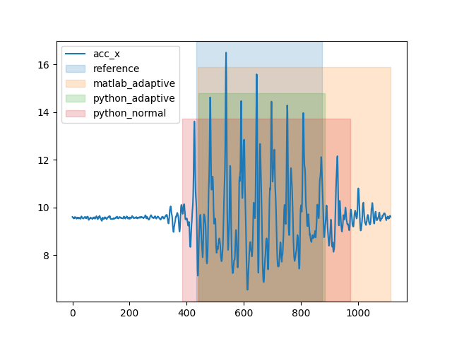
When we plot the output, we can see that the python version is more accurate and cuts the gait sequence roughly at the same time as the reference system, while the matlab version calssifies the small movement after the gait sequence as a gait as well.
fig, ax = plot_gsd_outputs(
    short_trial.data_ss,
    reference=short_trial_reference_parameters,
    matlab_adaptive=short_trial_matlab_output,
    python_adaptive=short_trial_output_adaptive.gs_list_,
    python_normal=short_trial_output_normal.gs_list_,
)
fig.show()
Performance on a longer lab trial#
Below we apply the algorithm to a lab trail that contains activities of daily living. This is a more challenging scenario, as we expect multiple gait sequences.
long_trial = lab_example_data.get_subset(
    cohort="MS", participant_id="001", test="Test11", trial="Trial1"
)
long_trial_matlab_output = load_matlab_output(long_trial)
long_trial_reference_parameters = long_trial.reference_parameters_.wb_list

long_trial_output_normal = GsdIonescu().detect(
    long_trial.data_ss, sampling_rate_hz=long_trial.sampling_rate_hz
)
long_trial_output_adaptive = GsdAdaptiveIonescu().detect(
    long_trial.data_ss, sampling_rate_hz=long_trial.sampling_rate_hz
)

print("Reference Parameters:\n\n", long_trial_reference_parameters)
print("\nMatlab Adaptive Ionescu Output:\n\n", long_trial_matlab_output)
print("\nPython Normal Ionescu Output:\n\n", long_trial_output_normal.gs_list_)
print(
    "\nPython Adaptive Ionescu Output:\n\n", long_trial_output_adaptive.gs_list_
)
/home/docs/checkouts/readthedocs.org/user_builds/mobgap/checkouts/v0.9.0/mobgap/data/_mobilised_matlab_loader.py:1082: UserWarning: There were multiple ICs with the same index value, but different LR labels. This is likely an issue with the reference system you should further investigate. For now, we set the `lr_label` of the stride corresponding to this IC to Nan. However, both values still remain in the IC list.
  return parse_reference_parameters(
Reference Parameters:

        start    end  ...  avg_stride_length_m  termination_reason
wb_id                ...
0       1019   1768  ...             0.942678               Pause
1       4534   5549  ...             0.483923               Pause
2       9665  10569  ...             0.506458               Pause
3      12337  14633  ...             0.803933               Pause
4      20151  20982  ...             0.507484               Pause
5      21378  22129  ...             0.599360               Pause

[6 rows x 9 columns]

Matlab Adaptive Ionescu Output:

    start    end
0    807   1842
1   5205   6010
2   9545  10620
3  12988  14670
4  20085  22728

Python Normal Ionescu Output:

        start    end
gs_id
0        847   1940
1       5202   6052
2       9585  10675
3      12952  14725
4      20235  22475

Python Adaptive Ionescu Output:

        start    end
gs_id
0        802   2032
1       4485   6092
2       9552  10730
3      11402  12040
4      12882  14752
5      19952  22507
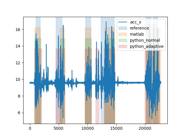
When we plot the output, we can see that the python version is more sensitive. It detects longer gait sequences and even one entire gait sequence that is not detected by the matlab version. But, like before, the Python version seems to provide the better results when compared to the reference system.
fig, _ = plot_gsd_outputs(
    long_trial.data_ss,
    reference=long_trial_reference_parameters,
    matlab=long_trial_matlab_output,
    python_normal=long_trial_output_normal.gs_list_,
    python_adaptive=long_trial_output_adaptive.gs_list_,
)
fig.show()
Evaluation of the algorithm against a reference#
To quantify how the Python output compares to the reference labels, we are providing a range of evaluation functions. See the example on GSD evaluation for more details.
Total running time of the script: (0 minutes 1.720 seconds)
Estimated memory usage: 9 MB