Gaussian Smoothing

A common low-pass filtering technique is Gaussian smoothing, which applies a Gaussian window to the data with a moving average. We provide a class based implementation of Gaussian smoothing in the GaussianFilter class.

import matplotlib.pyplot as plt
from mobgap.data import LabExampleDataset
from mobgap.data_transform import GaussianFilter

Loading some example data

example_data = LabExampleDataset()
ha_example_data = example_data.get_subset(cohort="HA")
single_test = ha_example_data.get_subset(
    participant_id="002", test="Test5", trial="Trial2"
)
data = single_test.data_ss

data.head()

	acc_x	acc_y	acc_z	gyr_x	gyr_y	gyr_z
time
2020-08-21 10:30:50.479000092+00:00	9.257165	0.031602	-2.604847	-0.1608	0.2119	-0.3052
2020-08-21 10:30:50.489000082+00:00	9.268460	0.017997	-2.594873	-0.2712	-0.0757	-0.4693
2020-08-21 10:30:50.499000072+00:00	9.272030	0.040954	-2.617060	0.1157	-0.0892	-0.2648
2020-08-21 10:30:50.509000063+00:00	9.262215	0.046100	-2.615381	-0.0091	-0.2005	-0.3278
2020-08-21 10:30:50.519000052+00:00	9.267278	0.070575	-2.585830	0.0524	-0.2733	-0.0965

Applying the Gaussian filter

We need to specify the standard deviation of the Gaussian window. Note, that we need to specify the standard deviation in seconds to make the parameters of the filter independent of the sampling rate of the data. It will be converted to samples internally.

gaussian_filter = GaussianFilter(sigma_s=0.1)
gaussian_filter.filter(data, sampling_rate_hz=single_test.sampling_rate_hz)
filtered_data = gaussian_filter.filtered_data_

filtered_data.head()

	acc_x	acc_y	acc_z	gyr_x	gyr_y	gyr_z
time
2020-08-21 10:30:50.479000092+00:00	9.257966	0.049992	-2.595191	0.290325	0.183090	-0.257459
2020-08-21 10:30:50.489000082+00:00	9.257946	0.050103	-2.595061	0.293245	0.185868	-0.257351
2020-08-21 10:30:50.499000072+00:00	9.257907	0.050325	-2.594804	0.299015	0.191387	-0.257147
2020-08-21 10:30:50.509000063+00:00	9.257853	0.050657	-2.594423	0.307482	0.199569	-0.256873
2020-08-21 10:30:50.519000052+00:00	9.257789	0.051097	-2.593921	0.318430	0.210298	-0.256555

We can also access the standard deviation in samples that was calculated from the provided sigma_s and the sampling rate.

gaussian_filter.sigma_samples_

10.0

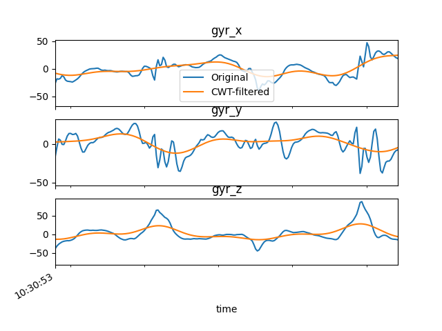
We will plot the filtered data together with the original data.

fig, axs = plt.subplots(3, 1, sharex=True)
for ax, col in zip(axs, ["gyr_x", "gyr_y", "gyr_z"]):
    ax.set_title(col)
    data[col].plot(ax=ax, label="Original")
    filtered_data[col].plot(ax=ax, label="CWT-filtered")

axs[0].set_xlim(data.index[300], data.index[500])
axs[0].legend()
fig.show()

Estimated memory usage: 9 MB