Note
Go to the end to download the full example code.
Performance of the initial contact algorithms on the TVS dataset#
The following provides an analysis and comparison of the icd performance on the TVS dataset (lab and free-living). We look into the actual performance of the algorithms compared to the reference data and compare these results with the performance of the original matlab algorithm.
Note
If you are interested in how these results are calculated, head over to the processing page.
We focus on the single_results (aka the performance per trail) and will aggregate it over multiple levels.
Below are the list of algorithms that we will compare. Note, that we use the prefix “MobGap” to refer to the reimplemented python algorithms and “Original Implementation” to refer to the original matlab algorithms.
# Note also that the IcdIonescu algorithm is the reimplementation of the Ani_McCamley algorithm in the original
# matlab algorithms.
# The  other two algorithms (IcdShinImproved and IcdHKLeeImproved) are actually cadence algorithms.
# As they can also be used to detect initial contacts, we present their results as well.
# However, you should check the dedicated cadence analysis for a more detailed comparison of these algorithms.
algorithms = {
    "IcdIonescu": ("IcdIonescu", "MobGap"),
    "IcdShinImproved": ("IcdShinImproved", "MobGap"),
    "IcdHKLeeImproved": ("IcdHKLeeImproved", "MobGap"),
}
# We only load the matlab algorithms that we reimplemented
algorithms.update(
    {
        "matlab_Ani_McCamley": ("IcdIonescu", "Original Implementation"),
    }
)
The code below loads the data and prepares it for the analysis.
By default, the data will be downloaded from an online repository (and cached locally).
If you want to use a local copy of the data, you can set the MOBGAP_VALIDATION_DATA_PATH environment variable.
and the MOBGAP_VALIDATION_USE_LOCA_DATA to 1.
The file download will print a couple log information, which can usually be ignored.
You can also change the version parameter to load a different version of the data.
from pathlib import Path

import pandas as pd
from mobgap.data.validation_results import ValidationResultLoader
from mobgap.utils.misc import get_env_var

local_data_path = (
    Path(get_env_var("MOBGAP_VALIDATION_DATA_PATH")) / "results"
    if int(get_env_var("MOBGAP_VALIDATION_USE_LOCAL_DATA", 0))
    else None
)
__RESULT_VERSION = "v1.2.0"
loader = ValidationResultLoader(
    "icd", result_path=local_data_path, version=__RESULT_VERSION
)

free_living_index_cols = [
    "cohort",
    "participant_id",
    "time_measure",
    "recording",
    "recording_name",
    "recording_name_pretty",
]

results = {
    v: loader.load_single_results(k, "free_living")
    for k, v in algorithms.items()
}
results = pd.concat(results, names=["algo", "version", *free_living_index_cols])
results_long = results.reset_index().assign(
    algo_with_version=lambda df: df["algo"] + " (" + df["version"] + ")",
    _combined="combined",
)

lab_index_cols = [
    "cohort",
    "participant_id",
    "time_measure",
    "test",
    "trial",
    "test_name",
    "test_name_pretty",
]

lab_results = {
    v: loader.load_single_results(k, "laboratory")
    for k, v in algorithms.items()
}
lab_results = pd.concat(lab_results, names=["algo", "version", *lab_index_cols])
lab_results_long = lab_results.reset_index().assign(
    algo_with_version=lambda df: df["algo"] + " (" + df["version"] + ")",
    _combined="combined",
)

cohort_order = ["HA", "CHF", "COPD", "MS", "PD", "PFF"]
  0%|                                              | 0.00/5.94k [00:00<?, ?B/s]
  0%|                                              | 0.00/5.94k [00:00<?, ?B/s]
100%|█████████████████████████████████████| 5.94k/5.94k [00:00<00:00, 29.7MB/s]

  0%|                                              | 0.00/5.94k [00:00<?, ?B/s]
  0%|                                              | 0.00/5.94k [00:00<?, ?B/s]
100%|█████████████████████████████████████| 5.94k/5.94k [00:00<00:00, 34.9MB/s]

  0%|                                              | 0.00/5.97k [00:00<?, ?B/s]
  0%|                                              | 0.00/5.97k [00:00<?, ?B/s]
100%|█████████████████████████████████████| 5.97k/5.97k [00:00<00:00, 33.4MB/s]

  0%|                                              | 0.00/5.91k [00:00<?, ?B/s]
  0%|                                              | 0.00/5.91k [00:00<?, ?B/s]
100%|█████████████████████████████████████| 5.91k/5.91k [00:00<00:00, 29.1MB/s]

  0%|                                              | 0.00/25.7k [00:00<?, ?B/s]
  0%|                                              | 0.00/25.7k [00:00<?, ?B/s]
100%|██████████████████████████████████████| 25.7k/25.7k [00:00<00:00, 121MB/s]

  0%|                                              | 0.00/25.8k [00:00<?, ?B/s]
  0%|                                              | 0.00/25.8k [00:00<?, ?B/s]
100%|██████████████████████████████████████| 25.8k/25.8k [00:00<00:00, 140MB/s]

  0%|                                              | 0.00/25.9k [00:00<?, ?B/s]
  0%|                                              | 0.00/25.9k [00:00<?, ?B/s]
100%|██████████████████████████████████████| 25.9k/25.9k [00:00<00:00, 137MB/s]

  0%|                                              | 0.00/25.2k [00:00<?, ?B/s]
  0%|                                              | 0.00/25.2k [00:00<?, ?B/s]
100%|██████████████████████████████████████| 25.2k/25.2k [00:00<00:00, 142MB/s]
Performance metrics#
For each participant, performance metrics were calculated by classifying the detected initial contacts as TP, FP or FN matches. Based on these values, recall (sensitivity), precision (positive predictive value), F1 score were calculated. On top of that, absolute error for each true positive initial contact was calculated as the temporal difference between detected and reference values. Relative error was calculated by dividing all absolute errors, within a walking bout, by the average step duration estimated from the reference system. From these, we calculate the mean and confidence interval for both systems, the bias and limits of agreement (LoA) between the algorithm output and the reference data, and the ICC.
Below the functions that calculate these metrics are defined.
from functools import partial

from mobgap.pipeline.evaluation import CustomErrorAggregations as A
from mobgap.utils.df_operations import (
    CustomOperation,
    apply_aggregations,
    apply_transformations,
    multilevel_groupby_apply_merge,
)
from mobgap.utils.tables import FormatTransformer as F
from mobgap.utils.tables import RevalidationInfo, revalidation_table_styles
from mobgap.utils.tables import StatsFunctions as S

custom_aggs = [
    CustomOperation(
        identifier=None,
        function=A.n_datapoints,
        column_name=[("n_datapoints", "all")],
    ),
    ("recall", ["mean", A.conf_intervals]),
    ("precision", ["mean", A.conf_intervals]),
    ("f1_score", ["mean", A.conf_intervals]),
    ("tp_absolute_timing_error_s", ["mean", A.loa]),
    ("tp_relative_timing_error", ["mean", A.loa]),
]

stats_transform = [
    CustomOperation(
        identifier=None,
        function=partial(
            S.pairwise_tests,
            value_col=c,
            between="version",
            reference_group_key="Original Implementation",
        ),
        column_name=[("stats_metadata", c)],
    )
    for c in [
        "recall",
        "precision",
        "f1_score",
    ]
]

format_transforms = [
    CustomOperation(
        identifier=None,
        function=lambda df_: df_[("n_datapoints", "all")].astype(int),
        column_name=("General", "n_datapoints"),
    ),
    *(
        CustomOperation(
            identifier=None,
            function=partial(
                F.value_with_metadata,
                value_col=("mean", c),
                other_columns={
                    "range": ("conf_intervals", c),
                    "stats_metadata": ("stats_metadata", c),
                },
            ),
            column_name=("ICD", c),
        )
        for c in [
            "recall",
            "precision",
            "f1_score",
        ]
    ),
    *(
        CustomOperation(
            identifier=None,
            function=partial(
                F.value_with_metadata,
                value_col=("mean", c),
                other_columns={"range": ("loa", c)},
            ),
            column_name=("IC Timing", c),
        )
        for c in [
            "tp_absolute_timing_error_s",
            "tp_relative_timing_error",
        ]
    ),
]

final_names = {
    "n_datapoints": "# recordings",
    "recall": "Recall",
    "precision": "Precision",
    "f1_score": "F1 Score",
    "tp_absolute_timing_error_s": "Abs. Error [s]",
    "tp_relative_timing_error": "Bias and LoA",
}


validation_thresholds = {
    ("ICD", "Recall"): RevalidationInfo(threshold=0.7, higher_is_better=True),
    ("ICD", "Precision"): RevalidationInfo(
        threshold=0.7, higher_is_better=True
    ),
    ("ICD", "F1 Score"): RevalidationInfo(threshold=0.7, higher_is_better=True),
}


def format_results(df: pd.DataFrame) -> pd.DataFrame:
    return (
        df.pipe(apply_transformations, format_transforms)
        .rename(columns=final_names)
        .loc[:, pd.IndexSlice[:, list(final_names.values())]]
    )
Free-Living Comparison#
We focus the comparison on the free-living data, as this is the most relevant considering our final use-case. In the free-living data, there is one 2.5 hour recording per participant. This means, each datapoint in the plots below and in the summary statistics represents one participant.
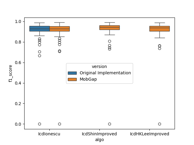
All results across all cohorts#
import matplotlib.pyplot as plt
import seaborn as sns

hue_order = ["Original Implementation", "MobGap"]

fig, ax = plt.subplots()
sns.boxplot(
    data=results_long,
    x="algo",
    y="f1_score",
    hue="version",
    hue_order=hue_order,
    ax=ax,
)
fig.show()

perf_metrics_all = results_long.pipe(
    multilevel_groupby_apply_merge,
    [
        (
            ["algo", "version"],
            partial(apply_aggregations, aggregations=custom_aggs),
        ),
        (
            ["algo"],
            partial(apply_transformations, transformations=stats_transform),
        ),
    ],
).pipe(format_results)
perf_metrics_all.style.pipe(
    revalidation_table_styles,
    validation_thresholds,
    ["algo"],
)
Per Cohort#
While this provides a good overview, it does not fully reflect how these algorithms perform on the different cohorts.
fig, ax = plt.subplots()
sns.boxplot(
    data=results_long, x="cohort", y="f1_score", hue="algo_with_version", ax=ax
)
fig.show()

perf_metrics_per_cohort = (
    results_long.pipe(
        multilevel_groupby_apply_merge,
        [
            (
                ["cohort", "algo", "version"],
                partial(apply_aggregations, aggregations=custom_aggs),
            ),
            (
                ["cohort", "algo"],
                partial(apply_transformations, transformations=stats_transform),
            ),
        ],
    )
    .pipe(format_results)
    .loc[cohort_order]
)
perf_metrics_per_cohort.style.pipe(
    revalidation_table_styles,
    validation_thresholds,
    ["cohort", "algo"],
)

Only relevant algorithms#
Finally, we present comparison of the old and new implementations of IcdIonescu. IcdShinImproved and IcdHKLeeImproved are excluded because they are cadence algorithms and we don’t calculate ICs with these algos in the old Matlab implementation.
fig, ax = plt.subplots()
sns.boxplot(
    data=results_long.query("algo == 'IcdIonescu'"),
    x="cohort",
    y="f1_score",
    hue="algo_with_version",
    ax=ax,
)
fig.show()

final_perf_metrics = (
    perf_metrics_per_cohort.copy()
    .query("algo == 'IcdIonescu'")
    .reset_index(level="algo", drop=True)
)

final_perf_metrics.style.pipe(
    revalidation_table_styles,
    validation_thresholds,
    ["cohort"],
)

Laboratory Comparison#
Every datapoint below is one trial of a test. Note, that each datapoint is weighted equally in the calculation of the performance metrics. This is a limitation of this simple approach, as the number of strides per trial and the complexity of the context can vary significantly. For a full picture, different groups of tests should be analyzed separately. The approach below should still provide a good overview to compare the algorithms.
hue_order = ["Original Implementation", "MobGap"]

fig, ax = plt.subplots()
sns.boxplot(
    data=lab_results_long,
    x="algo",
    y="f1_score",
    hue="version",
    hue_order=hue_order,
    ax=ax,
)
fig.show()

perf_metrics_all = lab_results_long.pipe(
    multilevel_groupby_apply_merge,
    [
        (
            ["algo", "version"],
            partial(apply_aggregations, aggregations=custom_aggs),
        ),
        (
            ["algo"],
            partial(apply_transformations, transformations=stats_transform),
        ),
    ],
).pipe(format_results)
perf_metrics_all.style.pipe(
    revalidation_table_styles,
    validation_thresholds,
    ["algo"],
)

Per Cohort#
While this provides a good overview, it does not fully reflect how these algorithms perform on the different cohorts.
fig, ax = plt.subplots()
sns.boxplot(
    data=lab_results_long,
    x="cohort",
    y="f1_score",
    hue="algo_with_version",
    ax=ax,
)
fig.show()

perf_metrics_per_cohort = (
    lab_results_long.pipe(
        multilevel_groupby_apply_merge,
        [
            (
                ["cohort", "algo", "version"],
                partial(apply_aggregations, aggregations=custom_aggs),
            ),
            (
                ["cohort", "algo"],
                partial(apply_transformations, transformations=stats_transform),
            ),
        ],
    )
    .pipe(format_results)
    .loc[cohort_order]
)
perf_metrics_per_cohort.style.pipe(
    revalidation_table_styles,
    validation_thresholds,
    ["cohort", "algo"],
)

Only relevant algorithms#
Finally, we present comparison of the old and new implementations of IcdIonescu. IcdShinImproved and IcdHKLeeImproved are excluded because they are cadence algorithms and we don’t calculate ICs with these algos in the old Matlab implementation.
fig, ax = plt.subplots()
sns.boxplot(
    data=lab_results_long.query("algo == 'IcdIonescu'"),
    x="cohort",
    y="f1_score",
    hue="algo_with_version",
    ax=ax,
)
fig.show()

final_perf_metrics = perf_metrics_per_cohort.query(
    "algo == 'IcdIonescu'"
).reset_index(level="algo", drop=True)

final_perf_metrics.style.pipe(
    revalidation_table_styles,
    validation_thresholds,
    ["cohort"],
)

Total running time of the script: (0 minutes 6.588 seconds)
Estimated memory usage: 81 MB