Note
Go to the end to download the full example code
LRC Evaluation#
This example demonstrates how to evaluate an LRC algorithm. As left-right classification, is a balanced binary classification problem, we can apply simple metrics like accuracy to evaluate the performance of the algorithm.
import pandas as pd

from mobgap.data import LabExampleDataset
from mobgap.lrc import LrcUllrich
from mobgap.pipeline import GsIterator
Loading some example data#
First, we load some example data and apply the LrcUllrich algorithm with its default pre-trained model to it. We use the reference initial contacts as input for the algorithm so that we can focus on the evaluation of the L/R classification independently of the detection of the initial contacts. However, you can use any other algorithm as well.
def load_data():
    lab_example_data = LabExampleDataset(reference_system="INDIP")
    single_test = lab_example_data.get_subset(cohort="MS", participant_id="001", test="Test11", trial="Trial1")
    return single_test


def calculate_output(single_test_data):
    """Calculate the GSD Iluz output per WB."""
    iterator = GsIterator()
    ref_paras = single_test_data.reference_parameters_relative_to_wb_

    for (gs, data), r in iterator.iterate(single_test_data.data_ss, ref_paras.wb_list):
        ref_ics = ref_paras.ic_list.loc[gs.id]
        r.ic_list = LrcUllrich().predict(data, ref_ics, sampling_rate_hz=single_test_data.sampling_rate_hz).ic_lr_list_

    return iterator.results_.ic_list


def load_reference(single_test_data):
    """Load the reference gait sequences from the test data."""
    ref_gsd = single_test_data.reference_parameters_.ic_list
    return ref_gsd


test_data = load_data()
calculated_ic_lr_list = calculate_output(test_data)
reference_ic_lr_list = load_reference(test_data)
We can see that the calculated and the reference ic_list have the same structure with the lr_label column
providing the detected label per initial contact.
Visual comparison of the detected and reference labels#
One easy way to compare the results is to visualize them as colorful bars.
import matplotlib.pyplot as plt


def plot_lr(ref, detected):
    fig, ax = plt.subplots(figsize=(15, 5))
    # We plot one box either (red or blue depending on the laterality) for each detected IC ignoring the actual time
    for (_, row), (_, ref_row) in zip(detected.iterrows(), ref.iterrows()):
        ax.plot([row["ic"], row["ic"]], [0, 0.98], color="r" if row["lr_label"] == "left" else "b", linewidth=5)
        ax.plot(
            [ref_row["ic"], ref_row["ic"]], [1.02, 2], color="r" if ref_row["lr_label"] == "left" else "b", linewidth=5
        )

    ax.set_yticks([0.5, 1.5])
    ax.set_yticklabels(["Detected", "Reference"])
    return fig, ax


fig, _ = plot_lr(reference_ic_lr_list, calculated_ic_lr_list)
fig.show()
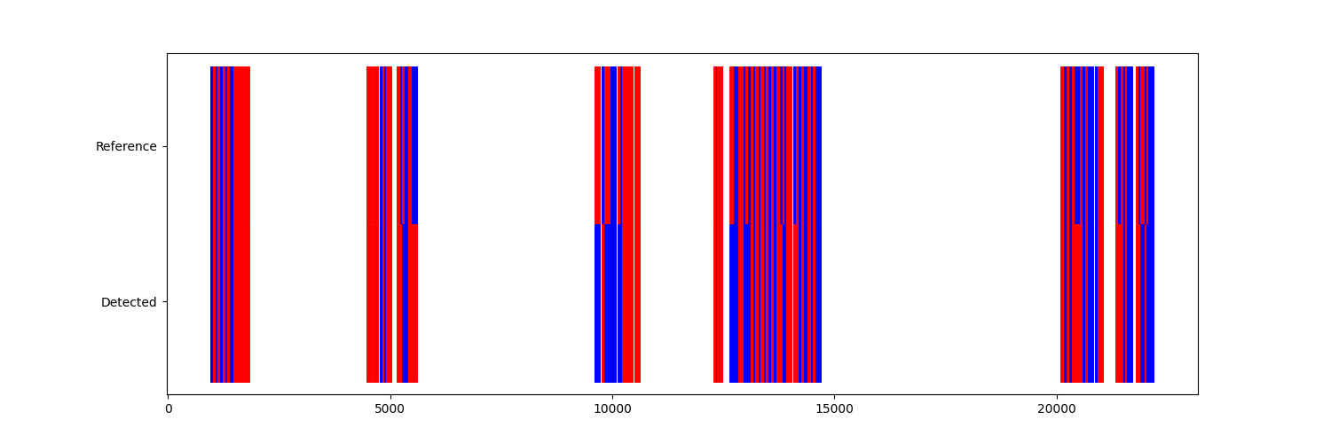
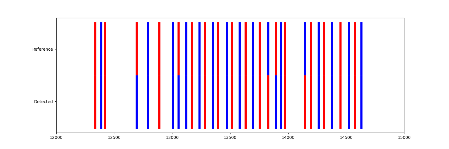
If we zoom in on a longer WB, we can see that for some ICs the L/R label does not match. But, in particular for regular gait in the center of the WB, the labels match quite well.
fig, ax = plot_lr(reference_ic_lr_list, calculated_ic_lr_list)
ax.set_xlim(12000, 15000)
fig.show()
Calculating evaluation metrics#
We can also quantify the agreement between the detected and the reference labels using typical classification metrics.
from sklearn.metrics import classification_report

pd.DataFrame(
    classification_report(
        reference_ic_lr_list["lr_label"],
        calculated_ic_lr_list["lr_label"],
        target_names=["left", "right"],
        output_dict=True,
    )
).T
In general we focus on the accuracy, as it is a balanced binary classification problem.
If you only want to calculate this you can just calculate the accuracy_score
from sklearn.metrics import accuracy_score

accuracy_score(reference_ic_lr_list["lr_label"], calculated_ic_lr_list["lr_label"])
0.7912087912087912
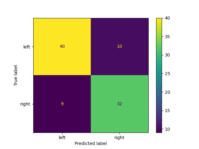
Similarly, we could create a confusion matrix to get more insights into the performance of the algorithm.
from sklearn.metrics import ConfusionMatrixDisplay

disp = ConfusionMatrixDisplay.from_predictions(reference_ic_lr_list["lr_label"], calculated_ic_lr_list["lr_label"])
disp.figure_.show()
Running a full evaluation pipeline#
Instead of manually evaluating and investigating the performance of an algorithm on a single piece of data, we
often want to run a full evaluation on an entire dataset.
This can be done using the LrdPipeline class and some tpcp functions.
But let’s start with selecting some data. We want to use all the simulated real-world walking data from the INDIP reference system (Test11).
simulated_real_world_walking = LabExampleDataset(reference_system="INDIP").get_subset(test="Test11")

simulated_real_world_walking
Now we can create a pipeline instance and directly run it on of the datapoints of the dataset.
from mobgap.lrc.pipeline import LrcEmulationPipeline

pipeline = LrcEmulationPipeline(LrcUllrich())

pipeline.safe_run(simulated_real_world_walking[0]).ic_lr_list_
This is exactly what we did before, just on a pipeline level, without manually extracting the data from the dataset.
To now actually run a validation, we need to iterate over all datapoints and calculate the accuracy for each of them.
This can be done using the validate function.
Note, that the LrdPipeline class already has a score method that returns the accuracy.
This is used by default, but you could supply your own scoring method as well.
from tpcp.validate import validate

evaluation_results_with_opti = pd.DataFrame(validate(pipeline, simulated_real_world_walking))
evaluation_results_with_opti.drop(["single_raw_results"], axis=1).T
Datapoints:   0%|          | 0/3 [00:00<?, ?it/s]
Datapoints:  33%|███▎      | 1/3 [00:00<00:01,  1.96it/s]
Datapoints:  67%|██████▋   | 2/3 [00:00<00:00,  2.15it/s]
Datapoints: 100%|██████████| 3/3 [00:01<00:00,  1.89it/s]
Datapoints: 100%|██████████| 3/3 [00:01<00:00,  1.94it/s]
The accuracy provided is the mean accuracy over all datapoints.
The accuracy per datapoint can be found in the single_accuracy column.
In addition to the metrics, we also provide the raw results for each datapoint in the single_raw_results column.
This could be used for further analysis.
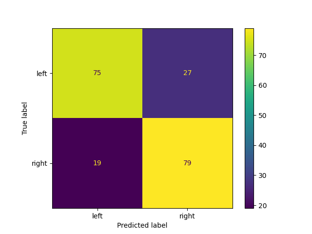
For example to calculate the confusion matrix over all ICs of all datapoints.
raw_results = pd.concat(
    evaluation_results_with_opti["single_raw_results"][0], keys=evaluation_results_with_opti["data_labels"][0], axis=0
)

raw_results.head()
The confusion matrix can be calculated using the same functions as before.
disp = ConfusionMatrixDisplay.from_predictions(raw_results["ref_lr_label"], raw_results["lr_label"])
disp.figure_.show()
If you want to calculate additional metrics, you can either create a custom score function or subclass the pipeline and overwrite the score function.
Parameter Optimization and Model Training#
Simply applying an algorithm for evaluation is one thing, but often we want to optimize the parameters of the algorithm, train internal models, or both and evalute the performance of this optimization approach and not just a fixed algorithm/model.
In this case, we need to create a train test split on the dataset and to ensure we have independent data for the
optimization.
In general, we would recommend using a cross-validation approach.
This can be done using the cross_validate function.
In the example below, we show the “most complicated” case, where we retrain the internal model of the LrcUllrich
algorithm and optimize one of the Hyperparmeters of the internal SVM.
As we retrain the model and optimize hyperparameters, we need to use a GridSearchCV nested
within the cross-validation loop.
Let’s set this up first.
from sklearn.model_selection import ParameterGrid
from sklearn.pipeline import Pipeline
from sklearn.preprocessing import MinMaxScaler
from sklearn.svm import SVC
from tpcp.optimize import GridSearchCV
We initialize the pipeline with an untrained model and an untrained scaler as a new pipeline.
clf_pipeline = Pipeline([("scaler", MinMaxScaler()), ("clf", SVC(kernel="linear"))])
pipeline = LrcEmulationPipeline(LrcUllrich(clf_pipe=clf_pipeline))
Then we can create a parameter Grid for the gridsearch.
Note, that we use __ to set nested parameters.
para_grid = ParameterGrid({"algo__clf_pipe__clf__C": [0.1, 1.0, 10.0]})
Then we path the pipeline to the optimizer. We only select a 2-fold cross-validation for this example, as we will only have 2 datapoints per train set and we want to minimize run time for this example.
optimizer = GridSearchCV(pipeline, para_grid, return_optimized="accuracy", cv=2)
Let’s test the optimizer first on a manual train set.
Split-Para Combos:   0%|          | 0/6 [00:00<?, ?it/s]

Datapoints:   0%|          | 0/1 [00:00<?, ?it/s]

Datapoints: 100%|██████████| 1/1 [00:00<00:00,  2.02it/s]
Datapoints: 100%|██████████| 1/1 [00:00<00:00,  2.02it/s]

Split-Para Combos:  17%|█▋        | 1/6 [00:00<00:04,  1.03it/s]

Datapoints:   0%|          | 0/1 [00:00<?, ?it/s]

Datapoints: 100%|██████████| 1/1 [00:00<00:00,  2.34it/s]
Datapoints: 100%|██████████| 1/1 [00:00<00:00,  2.34it/s]

Split-Para Combos:  33%|███▎      | 2/6 [00:01<00:03,  1.05it/s]

Datapoints:   0%|          | 0/1 [00:00<?, ?it/s]

Datapoints: 100%|██████████| 1/1 [00:00<00:00,  2.05it/s]
Datapoints: 100%|██████████| 1/1 [00:00<00:00,  2.05it/s]

Split-Para Combos:  50%|█████     | 3/6 [00:02<00:02,  1.05it/s]

Datapoints:   0%|          | 0/1 [00:00<?, ?it/s]

Datapoints: 100%|██████████| 1/1 [00:00<00:00,  2.37it/s]
Datapoints: 100%|██████████| 1/1 [00:00<00:00,  2.37it/s]

Split-Para Combos:  67%|██████▋   | 4/6 [00:03<00:01,  1.06it/s]

Datapoints:   0%|          | 0/1 [00:00<?, ?it/s]

Datapoints: 100%|██████████| 1/1 [00:00<00:00,  2.03it/s]
Datapoints: 100%|██████████| 1/1 [00:00<00:00,  2.03it/s]

Split-Para Combos:  83%|████████▎ | 5/6 [00:04<00:00,  1.05it/s]

Datapoints:   0%|          | 0/1 [00:00<?, ?it/s]

Datapoints: 100%|██████████| 1/1 [00:00<00:00,  2.40it/s]
Datapoints: 100%|██████████| 1/1 [00:00<00:00,  2.40it/s]

Split-Para Combos: 100%|██████████| 6/6 [00:05<00:00,  1.06it/s]
Split-Para Combos: 100%|██████████| 6/6 [00:05<00:00,  1.05it/s]

GridSearchCV(cv=2, n_jobs=None, optimize_with_info=True, parameter_grid=<sklearn.model_selection._search.ParameterGrid object at 0x7fc76fc2ab00>, pipeline=LrcEmulationPipeline(algo=LrcUllrich(clf_pipe=Pipeline(steps=[('scaler', MinMaxScaler()), ('clf', SVC(kernel='linear'))]), smoothing_filter=ButterworthFilter(cutoff_freq_hz=(0.5, 2), filter_type='bandpass', order=4, zero_phase=True))), pre_dispatch='n_jobs', progress_bar=True, pure_parameters=False, return_optimized='accuracy', return_train_score=False, safe_optimize=True, scoring=None, verbose=0)
We can inspect the results:
results = pd.DataFrame(optimizer.cv_results_)
results.loc[:, ~results.columns.str.endswith("raw_results")].T
And apply/score the best performing and retrained model directly on the test set.
optimizer.score(simulated_real_world_walking[2])["accuracy"]
0.8681318681318682
Let’s run everything combined with the external cross-validate to actually validate our optimization approach.
from tpcp.validate import cross_validate

evaluation_results_with_opti = pd.DataFrame(cross_validate(optimizer, simulated_real_world_walking, cv=3))
evaluation_results_with_opti.loc[:, ~evaluation_results_with_opti.columns.str.endswith("raw_results")].T
CV Folds:   0%|          | 0/3 [00:00<?, ?it/s]

Split-Para Combos:   0%|          | 0/6 [00:00<?, ?it/s]


Datapoints:   0%|          | 0/1 [00:00<?, ?it/s]


Datapoints: 100%|██████████| 1/1 [00:00<00:00,  2.38it/s]
Datapoints: 100%|██████████| 1/1 [00:00<00:00,  2.37it/s]


Split-Para Combos:  17%|█▋        | 1/6 [00:01<00:05,  1.04s/it]


Datapoints:   0%|          | 0/1 [00:00<?, ?it/s]


Datapoints: 100%|██████████| 1/1 [00:00<00:00,  1.75it/s]
Datapoints: 100%|██████████| 1/1 [00:00<00:00,  1.75it/s]


Split-Para Combos:  33%|███▎      | 2/6 [00:02<00:04,  1.04s/it]


Datapoints:   0%|          | 0/1 [00:00<?, ?it/s]


Datapoints: 100%|██████████| 1/1 [00:00<00:00,  2.40it/s]
Datapoints: 100%|██████████| 1/1 [00:00<00:00,  2.40it/s]


Split-Para Combos:  50%|█████     | 3/6 [00:03<00:03,  1.03s/it]


Datapoints:   0%|          | 0/1 [00:00<?, ?it/s]


Datapoints: 100%|██████████| 1/1 [00:00<00:00,  1.75it/s]
Datapoints: 100%|██████████| 1/1 [00:00<00:00,  1.75it/s]


Split-Para Combos:  67%|██████▋   | 4/6 [00:04<00:02,  1.03s/it]


Datapoints:   0%|          | 0/1 [00:00<?, ?it/s]


Datapoints: 100%|██████████| 1/1 [00:00<00:00,  2.30it/s]
Datapoints: 100%|██████████| 1/1 [00:00<00:00,  2.30it/s]


Split-Para Combos:  83%|████████▎ | 5/6 [00:05<00:01,  1.04s/it]


Datapoints:   0%|          | 0/1 [00:00<?, ?it/s]


Datapoints: 100%|██████████| 1/1 [00:00<00:00,  1.72it/s]
Datapoints: 100%|██████████| 1/1 [00:00<00:00,  1.72it/s]


Split-Para Combos: 100%|██████████| 6/6 [00:06<00:00,  1.04s/it]
Split-Para Combos: 100%|██████████| 6/6 [00:06<00:00,  1.04s/it]


Datapoints:   0%|          | 0/1 [00:00<?, ?it/s]

Datapoints: 100%|██████████| 1/1 [00:00<00:00,  2.09it/s]
Datapoints: 100%|██████████| 1/1 [00:00<00:00,  2.08it/s]

CV Folds:  33%|███▎      | 1/3 [00:07<00:15,  7.82s/it]

Split-Para Combos:   0%|          | 0/6 [00:00<?, ?it/s]


Datapoints:   0%|          | 0/1 [00:00<?, ?it/s]


Datapoints: 100%|██████████| 1/1 [00:00<00:00,  2.06it/s]
Datapoints: 100%|██████████| 1/1 [00:00<00:00,  2.06it/s]


Split-Para Combos:  17%|█▋        | 1/6 [00:01<00:05,  1.09s/it]


Datapoints:   0%|          | 0/1 [00:00<?, ?it/s]


Datapoints: 100%|██████████| 1/1 [00:00<00:00,  1.74it/s]
Datapoints: 100%|██████████| 1/1 [00:00<00:00,  1.74it/s]


Split-Para Combos:  33%|███▎      | 2/6 [00:02<00:04,  1.09s/it]


Datapoints:   0%|          | 0/1 [00:00<?, ?it/s]


Datapoints: 100%|██████████| 1/1 [00:00<00:00,  2.06it/s]
Datapoints: 100%|██████████| 1/1 [00:00<00:00,  2.06it/s]


Split-Para Combos:  50%|█████     | 3/6 [00:03<00:03,  1.09s/it]


Datapoints:   0%|          | 0/1 [00:00<?, ?it/s]


Datapoints: 100%|██████████| 1/1 [00:00<00:00,  1.73it/s]
Datapoints: 100%|██████████| 1/1 [00:00<00:00,  1.73it/s]


Split-Para Combos:  67%|██████▋   | 4/6 [00:04<00:02,  1.09s/it]


Datapoints:   0%|          | 0/1 [00:00<?, ?it/s]


Datapoints: 100%|██████████| 1/1 [00:00<00:00,  2.04it/s]
Datapoints: 100%|██████████| 1/1 [00:00<00:00,  2.04it/s]


Split-Para Combos:  83%|████████▎ | 5/6 [00:05<00:01,  1.09s/it]


Datapoints:   0%|          | 0/1 [00:00<?, ?it/s]


Datapoints: 100%|██████████| 1/1 [00:00<00:00,  1.74it/s]
Datapoints: 100%|██████████| 1/1 [00:00<00:00,  1.74it/s]


Split-Para Combos: 100%|██████████| 6/6 [00:06<00:00,  1.09s/it]
Split-Para Combos: 100%|██████████| 6/6 [00:06<00:00,  1.09s/it]


Datapoints:   0%|          | 0/1 [00:00<?, ?it/s]

Datapoints: 100%|██████████| 1/1 [00:00<00:00,  2.43it/s]
Datapoints: 100%|██████████| 1/1 [00:00<00:00,  2.42it/s]

CV Folds:  67%|██████▋   | 2/3 [00:15<00:07,  7.99s/it]

Split-Para Combos:   0%|          | 0/6 [00:00<?, ?it/s]


Datapoints:   0%|          | 0/1 [00:00<?, ?it/s]


Datapoints: 100%|██████████| 1/1 [00:00<00:00,  2.04it/s]
Datapoints: 100%|██████████| 1/1 [00:00<00:00,  2.04it/s]


Split-Para Combos:  17%|█▋        | 1/6 [00:00<00:04,  1.06it/s]


Datapoints:   0%|          | 0/1 [00:00<?, ?it/s]


Datapoints: 100%|██████████| 1/1 [00:00<00:00,  2.39it/s]
Datapoints: 100%|██████████| 1/1 [00:00<00:00,  2.39it/s]


Split-Para Combos:  33%|███▎      | 2/6 [00:01<00:03,  1.06it/s]


Datapoints:   0%|          | 0/1 [00:00<?, ?it/s]


Datapoints: 100%|██████████| 1/1 [00:00<00:00,  2.07it/s]
Datapoints: 100%|██████████| 1/1 [00:00<00:00,  2.07it/s]


Split-Para Combos:  50%|█████     | 3/6 [00:02<00:02,  1.06it/s]


Datapoints:   0%|          | 0/1 [00:00<?, ?it/s]


Datapoints: 100%|██████████| 1/1 [00:00<00:00,  2.40it/s]
Datapoints: 100%|██████████| 1/1 [00:00<00:00,  2.39it/s]


Split-Para Combos:  67%|██████▋   | 4/6 [00:03<00:01,  1.06it/s]


Datapoints:   0%|          | 0/1 [00:00<?, ?it/s]


Datapoints: 100%|██████████| 1/1 [00:00<00:00,  2.03it/s]
Datapoints: 100%|██████████| 1/1 [00:00<00:00,  2.03it/s]


Split-Para Combos:  83%|████████▎ | 5/6 [00:04<00:00,  1.06it/s]


Datapoints:   0%|          | 0/1 [00:00<?, ?it/s]


Datapoints: 100%|██████████| 1/1 [00:00<00:00,  2.38it/s]
Datapoints: 100%|██████████| 1/1 [00:00<00:00,  2.38it/s]


Split-Para Combos: 100%|██████████| 6/6 [00:05<00:00,  1.06it/s]
Split-Para Combos: 100%|██████████| 6/6 [00:05<00:00,  1.06it/s]


Datapoints:   0%|          | 0/1 [00:00<?, ?it/s]

Datapoints: 100%|██████████| 1/1 [00:00<00:00,  1.72it/s]
Datapoints: 100%|██████████| 1/1 [00:00<00:00,  1.72it/s]

CV Folds: 100%|██████████| 3/3 [00:23<00:00,  7.65s/it]
CV Folds: 100%|██████████| 3/3 [00:23<00:00,  7.73s/it]
We can compare these results with the performance of the pre-trained model that was not optimized for the given
dataset, by using DummyOptimize, to run a cross-validation, but without any optimization.
We simply evaluate the pre-trained model on exactly the same test sets as the optimized model.
from tpcp.optimize import DummyOptimize

optimizer = DummyOptimize(LrcEmulationPipeline(LrcUllrich()))

evaluation_results_pre_trained = pd.DataFrame(cross_validate(optimizer, simulated_real_world_walking, cv=3))
evaluation_results_pre_trained.loc[:, ~evaluation_results_pre_trained.columns.str.endswith("raw_results")].T
CV Folds:   0%|          | 0/3 [00:00<?, ?it/s]/home/docs/checkouts/readthedocs.org/user_builds/mobgap/envs/v0.3.0/lib/python3.10/site-packages/tpcp/_utils/_score.py:258: PotentialUserErrorWarning: You are using `DummyOptimize` with a pipeline that implements `self_optimize` and, hence, indicates that the pipeline can be optimized. `DummyOptimize` does never call this method and skips any optimization steps! Use `Optimize` if you actually want to optimize your pipeline.
  return optimizer.set_params(**hyperparas).optimize(data, **optimize_params)


Datapoints:   0%|          | 0/1 [00:00<?, ?it/s]

Datapoints: 100%|██████████| 1/1 [00:00<00:00,  1.96it/s]
Datapoints: 100%|██████████| 1/1 [00:00<00:00,  1.96it/s]

CV Folds:  33%|███▎      | 1/3 [00:00<00:01,  1.82it/s]/home/docs/checkouts/readthedocs.org/user_builds/mobgap/envs/v0.3.0/lib/python3.10/site-packages/tpcp/_utils/_score.py:258: PotentialUserErrorWarning: You are using `DummyOptimize` with a pipeline that implements `self_optimize` and, hence, indicates that the pipeline can be optimized. `DummyOptimize` does never call this method and skips any optimization steps! Use `Optimize` if you actually want to optimize your pipeline.
  return optimizer.set_params(**hyperparas).optimize(data, **optimize_params)


Datapoints:   0%|          | 0/1 [00:00<?, ?it/s]

Datapoints: 100%|██████████| 1/1 [00:00<00:00,  2.32it/s]
Datapoints: 100%|██████████| 1/1 [00:00<00:00,  2.32it/s]

CV Folds:  67%|██████▋   | 2/3 [00:01<00:00,  2.00it/s]/home/docs/checkouts/readthedocs.org/user_builds/mobgap/envs/v0.3.0/lib/python3.10/site-packages/tpcp/_utils/_score.py:258: PotentialUserErrorWarning: You are using `DummyOptimize` with a pipeline that implements `self_optimize` and, hence, indicates that the pipeline can be optimized. `DummyOptimize` does never call this method and skips any optimization steps! Use `Optimize` if you actually want to optimize your pipeline.
  return optimizer.set_params(**hyperparas).optimize(data, **optimize_params)


Datapoints:   0%|          | 0/1 [00:00<?, ?it/s]

Datapoints: 100%|██████████| 1/1 [00:00<00:00,  1.67it/s]
Datapoints: 100%|██████████| 1/1 [00:00<00:00,  1.67it/s]

CV Folds: 100%|██████████| 3/3 [00:01<00:00,  1.78it/s]
CV Folds: 100%|██████████| 3/3 [00:01<00:00,  1.82it/s]
Note that using only so little data is not a good idea in practice. There are many parameters, that you should tweak to make this a robust validation. However, this example should provide a good starting point for your own experiments.
Total running time of the script: (0 minutes 39.687 seconds)
Estimated memory usage: 21 MB