Note
Go to the end to download the full example code
GSD Iluz#
This example shows how to use the GSD Iluz algorithm and some examples on how the results compare to the original matlab implementation.
We start by defining some helpers for plotting and loading the data. You can skip them for now and jump directly to “Performance on a single lab trial”, if you just want to see how to apply the algorithm.
Plotting Helper#
We define a helper function to plot the results of the algorithm. Just ignore this function for now.
import matplotlib.pyplot as plt


def plot_gsd_outputs(data, **kwargs):
    fig, ax = plt.subplots()

    ax.plot(data["acc_x"].to_numpy(), label="acc_x")

    color_cycle = iter(plt.rcParams["axes.prop_cycle"])

    y_max = 1.1
    plot_props = [
        {"data": v, "label": k, "alpha": 0.2, "ymax": (y_max := y_max - 0.1), "color": next(color_cycle)["color"]}
        for k, v in kwargs.items()
    ]

    for props in plot_props:
        for gsd in props.pop("data").itertuples(index=False):
            ax.axvspan(gsd.start, gsd.end, label=props.pop("label", None), **props)

    ax.legend()
    return fig, ax
Loading some example data#
Note
More infos about data loading can be found in the data loading example.
We load example data from the lab dataset together with the INDIP reference system. We will use the INDIP “WB” output as ground truth. Note, that the “WB” (Walking Bout) output is further processed than a normal “Gait Sequence”. This means we expect Gait Sequences to contain some false positives compared to the “WB” output. However, a good gait sequence detection algorithm should have high sensitivity (i.e. contain all the “WBs” of the reference system).
import json

import pandas as pd

from mobgap import PACKAGE_ROOT
from mobgap.data import LabExampleDataset

lab_example_data = LabExampleDataset(reference_system="INDIP")


def load_matlab_output(datapoint):
    p = datapoint.group_label
    with (
        PACKAGE_ROOT.parent
        / f"example_data/original_results/gsd_iluz/lab/{p.cohort}/{p.participant_id}/GSDA_Output.json"
    ).open() as f:
        original_results = json.load(f)["GSDA_Output"][p.time_measure][p.test][p.trial]["SU"]["LowerBack"]["GSD"]

    if not isinstance(original_results, list):
        original_results = [original_results]
    return (
        pd.DataFrame.from_records(original_results).rename(
            {"GaitSequence_Start": "start", "GaitSequence_End": "end"}, axis=1
        )[["start", "end"]]
        * datapoint.sampling_rate_hz
    )
Performance on a single lab trial#
Below we apply the algorithm to a lab trail, where we only expect a single gait sequence.
from mobgap.gsd import GsdIluz

short_trial = lab_example_data.get_subset(cohort="HA", participant_id="001", test="Test5", trial="Trial2")
short_trial_matlab_output = load_matlab_output(short_trial)
short_trial_reference_parameters = short_trial.reference_parameters_.wb_list

short_trial_output = GsdIluz().detect(short_trial.data_ss, sampling_rate_hz=short_trial.sampling_rate_hz)

print("Reference Parameters:\n\n", short_trial_reference_parameters)
print("\nMatlab Output:\n\n", short_trial_matlab_output)
print("\nPython Output:\n\n", short_trial_output.gs_list_)
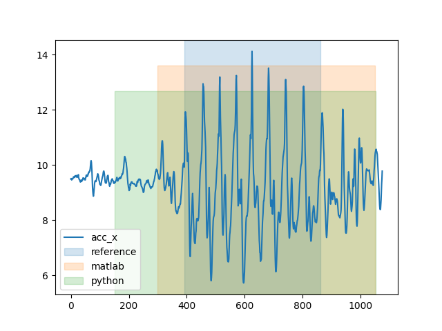
Reference Parameters:

        start  end  ...  avg_stride_length_m  termination_reason
wb_id              ...
1        392  862  ...             1.211187               Pause

[1 rows x 9 columns]

Matlab Output:

    start     end
0  299.0  1049.0

Python Output:

    start   end
0    150  1052
When we plot the output, we can see that the python version is a little more sensitive than the matlab version. It includes a section of the signal before the region classified as WB by the reference system. Both algorithm implementations produce a gait sequence that extends beyond the end of the reference system.
fig, ax = plot_gsd_outputs(
    short_trial.data_ss,
    reference=short_trial_reference_parameters,
    matlab=short_trial_matlab_output,
    python=short_trial_output.gs_list_,
)
fig.show()
Performance on a longer lab trial#
Below we apply the algorithm to a lab trail that contains activities of daily living. This is a more challenging scenario, as we expect multiple gait sequences.
long_trial = lab_example_data.get_subset(cohort="MS", participant_id="001", test="Test11", trial="Trial1")
long_trial_matlab_output = load_matlab_output(long_trial)
long_trial_reference_parameters = long_trial.reference_parameters_.wb_list

long_trial_output = GsdIluz().detect(long_trial.data_ss, sampling_rate_hz=long_trial.sampling_rate_hz)

print("Reference Parameters:\n\n", long_trial_reference_parameters)
print("\nMatlab Output:\n\n", long_trial_matlab_output)
print("\nPython Output:\n\n", long_trial_output.gs_list_)
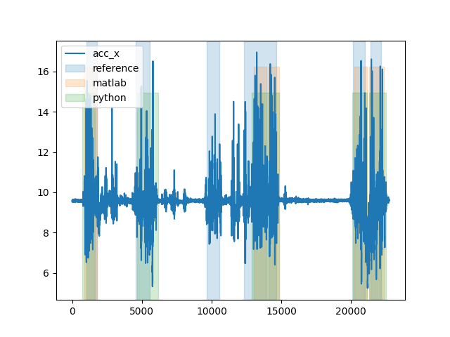
Reference Parameters:

        start    end  ...  avg_stride_length_m  termination_reason
wb_id                ...
1       1019   1768  ...             0.942678               Pause
2       4534   5549  ...             0.483923               Pause
3       9665  10569  ...             0.506458               Pause
4      12337  14633  ...             0.803933               Pause
5      20151  20982  ...             0.507484               Pause
6      21378  22129  ...             0.599360               Pause

[6 rows x 9 columns]

Matlab Output:

      start      end
0    899.0   1799.0
1  13049.0  13949.0
2  14099.0  14849.0
3  20249.0  21149.0
4  21299.0  22349.0

Python Output:

    start    end
0    750   1652
2   4650   6152
5  12900  14852
6  20100  21152
7  21300  22502
When we plot the output, we can see again that the python version is more sensitive. It detects longer gait sequences and even one entire gait sequence that is not detected by the matlab version.
fig, _ = plot_gsd_outputs(
    long_trial.data_ss,
    reference=long_trial_reference_parameters,
    matlab=long_trial_matlab_output,
    python=long_trial_output.gs_list_,
)
fig.show()
Changing the parameters#
The Python version aims to expose all relevant parameters of the algorithm.
The GsdlIluz algorithm has a lot of parameters that can be modified.
Finding a combination of parameters that works well for all scenarios is difficult.
Below we show, just how to modify them in general.
We modify one of the basic parameters, the window length. This can effect all parts of the output. In this case, we can see that all GSDs are slightly longer and that we now detect a gait sequence that was not detected before.
long_trial_output_modified = GsdIluz(window_length_s=5, window_overlap=0.8).detect(
    long_trial.data_ss, sampling_rate_hz=long_trial.sampling_rate_hz
)

print("Reference Parameters:\n\n", long_trial_reference_parameters)
print("\nPython Output:\n\n", long_trial_output.gs_list_)
print("\nPython Output Modified:\n\n", long_trial_output_modified.gs_list_)

fig, _ = plot_gsd_outputs(
    long_trial.data_ss,
    reference=long_trial_reference_parameters,
    python=long_trial_output.gs_list_,
    python_modified=long_trial_output_modified.gs_list_,
)
fig.show()
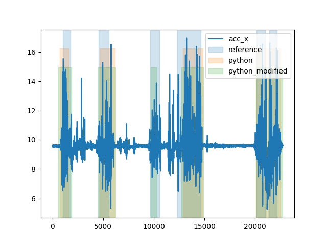
Reference Parameters:

        start    end  ...  avg_stride_length_m  termination_reason
wb_id                ...
1       1019   1768  ...             0.942678               Pause
2       4534   5549  ...             0.483923               Pause
3       9665  10569  ...             0.506458               Pause
4      12337  14633  ...             0.803933               Pause
5      20151  20982  ...             0.507484               Pause
6      21378  22129  ...             0.599360               Pause

[6 rows x 9 columns]

Python Output:

    start    end
0    750   1652
2   4650   6152
5  12900  14852
6  20100  21152
7  21300  22502

Python Output Modified:

    start    end
0    600   1902
1   4500   6202
2   9700  10302
3  12700  14902
4  20100  22702
Evaluation of the algorithm against a reference#
To quantify how the Python output compares to the reference labels, we are providing a range of evaluation functions. See the example on GSD evaluation for more details.
Total running time of the script: (0 minutes 4.628 seconds)
Estimated memory usage: 60 MB