Note
Go to the end to download the full example code.
Performance of the stride length algorithms on the TVS dataset#
The following provides an analysis and comparison of the stride length algorithms on the TVS dataset (lab and free-living). We look into the actual performance of the algorithms compared to the reference data and compare the results to the previous results generated by the matlab pipeline.
Note
If you are interested in how these results are calculated, head over to the processing page.
Below are the list of algorithms that we will compare. Note, that we use the prefix “MobGap” to refer to the reimplemented python algorithms. For the zjils algorithm, we compare both potential threshold values that were determined as part of the pre-validation analysis on the MsProject dataset.
algorithms = {
    "SlZjilstra__MS_ALL": ("SlZjilstra - MS-all", "MobGap"),
    "SlZjilstra__MS_MS": ("SlZjilstra - MS-MS", "MobGap"),
    "matlab_zjilsV3__MS_ALL": (
        "SlZjilstra - MS-all",
        "Original Implementation",
    ),
    "matlab_zjilsV3__MS_MS": ("SlZjilstra - MS-MS", "Original Implementation"),
}
The code below loads the data and prepares it for the analysis.
By default, the data will be downloaded from an online repository (and cached locally).
If you want to use a local copy of the data, you can set the MOBGAP_VALIDATION_DATA_PATH environment variable.
and the MOBGAP_VALIDATION_USE_LOCA_DATA to 1.
The file download will print a couple log information, which can usually be ignored.
You can also change the version parameter to load a different version of the data.
from pathlib import Path

import pandas as pd
from mobgap.data.validation_results import ValidationResultLoader
from mobgap.utils.misc import get_env_var


def format_loaded_results(
    values: dict[tuple[str, str], pd.DataFrame],
    index_cols: list[str],
    convert_rel_error: bool = False,
) -> pd.DataFrame:
    formatted = (
        pd.concat(values, names=["algo", "version", *index_cols])
        .reset_index()
        .assign(
            algo_with_version=lambda df: (
                df["algo"] + " (" + df["version"] + ")"
            ),
            _combined="combined",
        )
    )
    if not convert_rel_error:
        return formatted
    rel_cols = [c for c in formatted.columns if "rel_error" in c]
    formatted[rel_cols] = formatted[rel_cols] * 100
    return formatted


local_data_path = (
    Path(get_env_var("MOBGAP_VALIDATION_DATA_PATH")) / "results"
    if int(get_env_var("MOBGAP_VALIDATION_USE_LOCAL_DATA", 0))
    else None
)
__RESULT_VERSION = "v1.2.0"
loader = ValidationResultLoader(
    "sl", result_path=local_data_path, version=__RESULT_VERSION
)


free_living_index_cols = [
    "cohort",
    "participant_id",
    "time_measure",
    "recording",
    "recording_name",
    "recording_name_pretty",
]

free_living_results = format_loaded_results(
    {
        v: loader.load_single_results(k, "free_living")
        for k, v in algorithms.items()
    },
    free_living_index_cols,
    convert_rel_error=True,
)

lab_index_cols = [
    "cohort",
    "participant_id",
    "time_measure",
    "test",
    "trial",
    "test_name",
    "test_name_pretty",
]

lab_results = format_loaded_results(
    {
        v: loader.load_single_results(k, "laboratory")
        for k, v in algorithms.items()
    },
    lab_index_cols,
    convert_rel_error=True,
)

cohort_order = ["HA", "CHF", "COPD", "MS", "PD", "PFF"]
  0%|                                              | 0.00/12.0k [00:00<?, ?B/s]
  0%|                                              | 0.00/12.0k [00:00<?, ?B/s]
100%|█████████████████████████████████████| 12.0k/12.0k [00:00<00:00, 55.2MB/s]

  0%|                                              | 0.00/12.1k [00:00<?, ?B/s]
  0%|                                              | 0.00/12.1k [00:00<?, ?B/s]
100%|█████████████████████████████████████| 12.1k/12.1k [00:00<00:00, 86.0MB/s]

  0%|                                              | 0.00/11.9k [00:00<?, ?B/s]
  0%|                                              | 0.00/11.9k [00:00<?, ?B/s]
100%|█████████████████████████████████████| 11.9k/11.9k [00:00<00:00, 89.3MB/s]

  0%|                                              | 0.00/12.1k [00:00<?, ?B/s]
  0%|                                              | 0.00/12.1k [00:00<?, ?B/s]
100%|█████████████████████████████████████| 12.1k/12.1k [00:00<00:00, 90.1MB/s]

  0%|                                              | 0.00/89.6k [00:00<?, ?B/s]
  0%|                                              | 0.00/89.6k [00:00<?, ?B/s]
100%|██████████████████████████████████████| 89.6k/89.6k [00:00<00:00, 520MB/s]

  0%|                                              | 0.00/90.2k [00:00<?, ?B/s]
  0%|                                              | 0.00/90.2k [00:00<?, ?B/s]
100%|██████████████████████████████████████| 90.2k/90.2k [00:00<00:00, 549MB/s]

  0%|                                              | 0.00/87.5k [00:00<?, ?B/s]
  0%|                                              | 0.00/87.5k [00:00<?, ?B/s]
100%|██████████████████████████████████████| 87.5k/87.5k [00:00<00:00, 487MB/s]

  0%|                                              | 0.00/88.0k [00:00<?, ?B/s]
  0%|                                              | 0.00/88.0k [00:00<?, ?B/s]
100%|██████████████████████████████████████| 88.0k/88.0k [00:00<00:00, 519MB/s]
Performance metrics#
Below you can find the setup for all performance metrics that we will calculate.
We only use the wb__ results for the comparison.
These results are calculated by first calculating the average stride length per WB.
Then calculating the error metrics for each WB.
Then we take the average over all WBs of a participant to get the wb__ results.
from functools import partial

from mobgap.pipeline.evaluation import CustomErrorAggregations as A
from mobgap.utils.df_operations import (
    CustomOperation,
    apply_aggregations,
    apply_transformations,
    multilevel_groupby_apply_merge,
)
from mobgap.utils.tables import FormatTransformer as F
from mobgap.utils.tables import RevalidationInfo, revalidation_table_styles
from mobgap.utils.tables import StatsFunctions as S

custom_aggs = [
    CustomOperation(
        identifier=None,
        function=A.n_datapoints,
        column_name=[("n_datapoints", "all")],
    ),
    CustomOperation(
        identifier=None,
        function=lambda df_: df_["wb__detected"].isna().sum(),
        column_name=[("n_nan_detected", "all")],
    ),
    ("wb__detected", ["mean", A.conf_intervals]),
    ("wb__reference", ["mean", A.conf_intervals]),
    ("wb__error", ["mean", A.loa]),
    ("wb__abs_error", ["mean", A.conf_intervals]),
    ("wb__rel_error", ["mean", A.conf_intervals]),
    ("wb__abs_rel_error", ["mean", A.conf_intervals]),
    CustomOperation(
        identifier=None,
        function=partial(
            A.icc,
            reference_col_name="wb__reference",
            detected_col_name="wb__detected",
            icc_type="icc2",
            # For the lab data, some trials have no results for the old algorithms.
            nan_policy="omit",
        ),
        column_name=[("icc", "wb_level"), ("icc_ci", "wb_level")],
    ),
]

stats_transform = [
    CustomOperation(
        identifier=None,
        function=partial(
            S.pairwise_tests,
            value_col=c,
            between="version",
            reference_group_key="Original Implementation",
        ),
        column_name=[("stats_metadata", c)],
    )
    for c in [
        "wb__abs_error",
        "wb__abs_rel_error",
    ]
]

format_transforms = [
    CustomOperation(
        identifier=None,
        function=lambda df_: df_[("n_datapoints", "all")].astype(int),
        column_name="n_datapoints",
    ),
    CustomOperation(
        identifier=None,
        function=lambda df_: df_[("n_nan_detected", "all")].astype(int),
        column_name="n_nan_detected",
    ),
    *(
        CustomOperation(
            identifier=None,
            function=partial(
                F.value_with_metadata,
                value_col=("mean", c),
                other_columns={
                    "range": ("conf_intervals", c),
                    **(
                        {"stats_metadata": ("stats_metadata", c)}
                        if c in ["wb__abs_error", "wb__abs_rel_error"]
                        else {}
                    ),
                },
            ),
            column_name=c,
        )
        for c in [
            "wb__reference",
            "wb__detected",
            "wb__abs_error",
            "wb__rel_error",
            "wb__abs_rel_error",
        ]
    ),
    CustomOperation(
        identifier=None,
        function=partial(
            F.value_with_metadata,
            value_col=("mean", "wb__error"),
            other_columns={"range": ("loa", "wb__error")},
        ),
        column_name="wb__error",
    ),
    CustomOperation(
        identifier=None,
        function=partial(
            F.value_with_metadata,
            value_col=("icc", "wb_level"),
            other_columns={"range": ("icc_ci", "wb_level")},
        ),
        column_name="icc",
    ),
]


final_names = {
    "n_datapoints": "# participants",
    "wb__detected": "WD mean and CI [m]",
    "wb__reference": "INDIP mean and CI [m]",
    "wb__error": "Bias and LoA [m]",
    "wb__abs_error": "Abs. Error [m]",
    "wb__rel_error": "Rel. Error [%]",
    "wb__abs_rel_error": "Abs. Rel. Error [%]",
    "icc": "ICC",
    "n_nan_detected": "# Failed WBs",
}


validation_thresholds = {
    "Abs. Error [m]": RevalidationInfo(threshold=None, higher_is_better=False),
    "Abs. Rel. Error [%]": RevalidationInfo(
        threshold=20, higher_is_better=False
    ),
    "ICC": RevalidationInfo(threshold=0.7, higher_is_better=True),
    "# Failed WBs": RevalidationInfo(threshold=None, higher_is_better=False),
}


def format_tables(df: pd.DataFrame) -> pd.DataFrame:
    return (
        df.pipe(apply_transformations, format_transforms)
        .rename(columns=final_names)
        .loc[:, list(final_names.values())]
    )
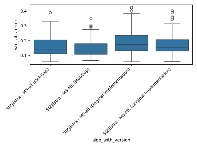
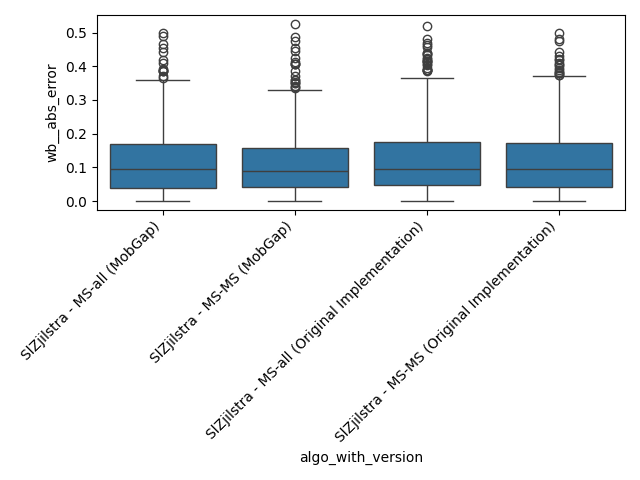
Free-Living Comparison#
We focus on the free-living data for the comparison as this is the expected use case for the algorithms.
All results across all cohorts#
The results below represent the average performance across all participants independent of the cohort.
import matplotlib.pyplot as plt
import seaborn as sns

fig, ax = plt.subplots()
sns.boxplot(
    data=free_living_results, x="algo_with_version", y="wb__abs_error", ax=ax
)
plt.xticks(rotation=45, ha="right")
fig.tight_layout()
fig.show()

perf_metrics_all = free_living_results.pipe(
    multilevel_groupby_apply_merge,
    [
        (
            ["algo", "version"],
            partial(apply_aggregations, aggregations=custom_aggs),
        ),
        (
            ["algo"],
            partial(apply_transformations, transformations=stats_transform),
        ),
    ],
).pipe(format_tables)
perf_metrics_all.style.pipe(
    revalidation_table_styles,
    validation_thresholds,
    ["algo"],
)
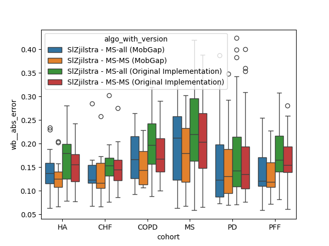
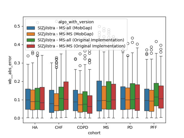
Per Cohort#
The results below represent the average performance across all participants within a cohort.
fig, ax = plt.subplots()
sns.boxplot(
    data=free_living_results,
    x="cohort",
    y="wb__abs_error",
    hue="algo_with_version",
    order=cohort_order,
    ax=ax,
)
fig.show()
perf_metrics_cohort = (
    free_living_results.pipe(
        multilevel_groupby_apply_merge,
        [
            (
                ["cohort", "algo", "version"],
                partial(apply_aggregations, aggregations=custom_aggs),
            ),
            (
                ["cohort", "algo"],
                partial(apply_transformations, transformations=stats_transform),
            ),
        ],
    )
    .pipe(format_tables)
    .loc[cohort_order]
)
perf_metrics_cohort.style.pipe(
    revalidation_table_styles,
    validation_thresholds,
    ["cohort", "algo"],
)
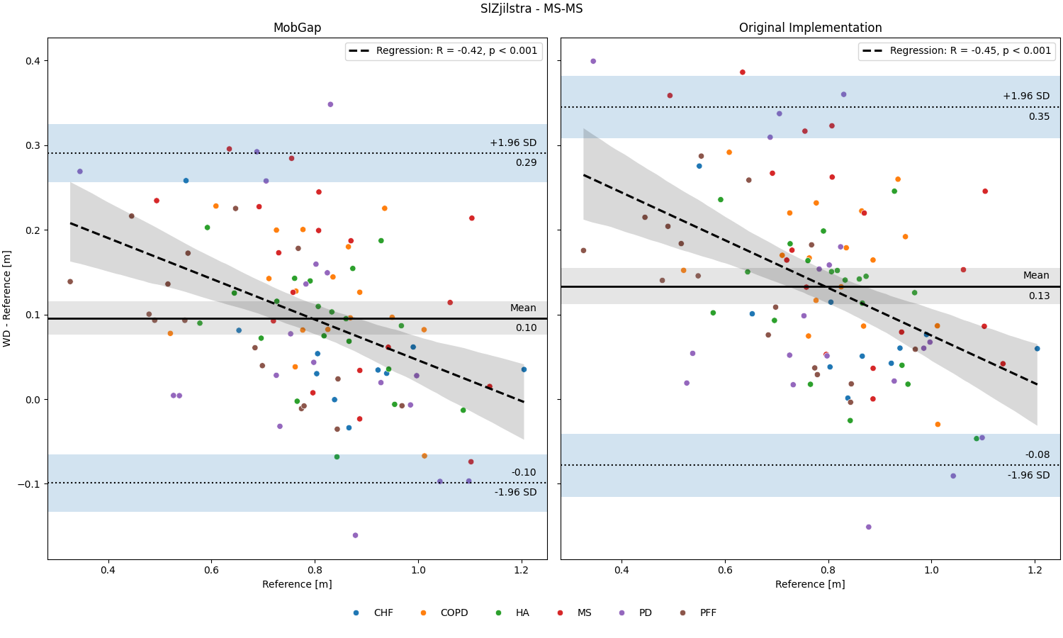
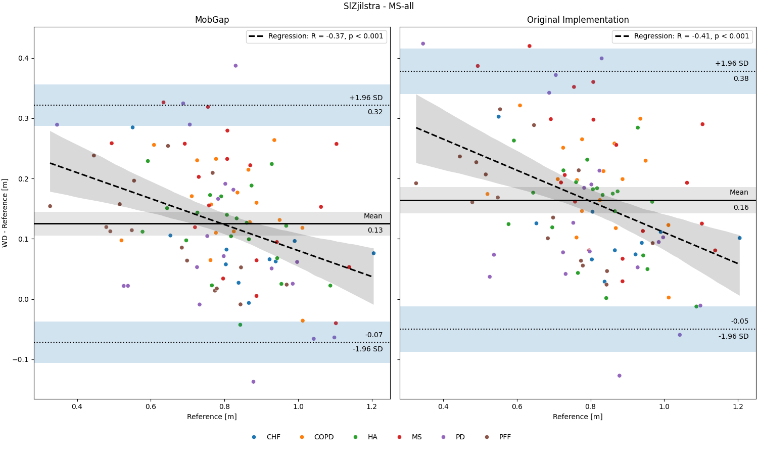
Deep Dive Analysis of Main Algorithms#
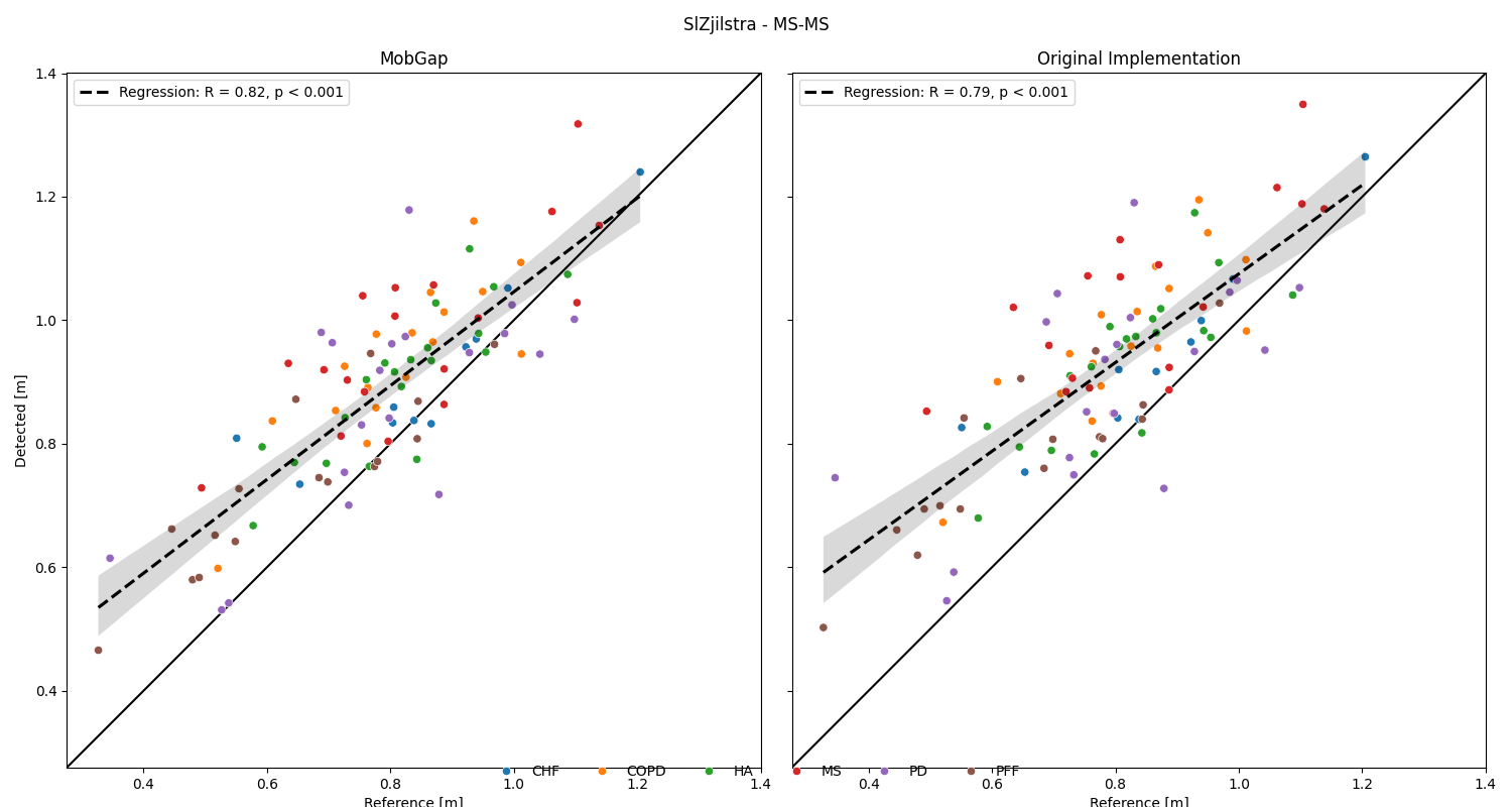
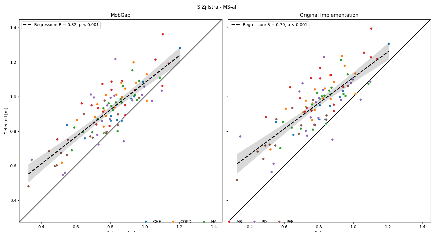
Below, you can find detailed correlation and residual plots comparing the new and the old implementation of each algorithm. Each datapoint represents one participant.
from mobgap.plotting import (
    calc_min_max_with_margin,
    make_square,
    move_legend_outside,
    plot_regline,
    residual_plot,
)


def combo_residual_plot(data):
    fig, axs = plt.subplots(
        ncols=2,
        sharey=True,
        sharex=True,
        figsize=(15, 9),
        constrained_layout=True,
    )
    fig.suptitle(data.name)
    for (version, subdata), ax in zip(data.groupby("version"), axs):
        residual_plot(
            subdata,
            "wb__reference",
            "wb__detected",
            "cohort",
            "m",
            ax=ax,
            legend=ax == axs[-1],
        )
        ax.set_title(version)
    move_legend_outside(fig, axs[-1])
    plt.show()


def combo_scatter_plot(data):
    fig, axs = plt.subplots(
        ncols=2,
        sharey=True,
        sharex=True,
        figsize=(15, 8),
        constrained_layout=True,
    )
    fig.suptitle(data.name)
    min_max = calc_min_max_with_margin(
        data["wb__reference"], data["wb__detected"]
    )
    for (version, subdata), ax in zip(data.groupby("version"), axs):
        subdata = subdata[["wb__reference", "wb__detected", "cohort"]].dropna(
            how="any"
        )
        sns.scatterplot(
            subdata,
            x="wb__reference",
            y="wb__detected",
            hue="cohort",
            ax=ax,
            legend=ax == axs[-1],
        )
        plot_regline(subdata["wb__reference"], subdata["wb__detected"], ax=ax)
        make_square(ax, min_max, draw_diagonal=True)
        ax.set_title(version)
        ax.set_xlabel("Reference [m]")
        ax.set_ylabel("Detected [m]")
    move_legend_outside(fig, axs[-1])
    plt.tight_layout()
    plt.show()


free_living_results.groupby("algo").apply(
    combo_residual_plot, include_groups=False
)
free_living_results.groupby("algo").apply(
    combo_scatter_plot, include_groups=False
)
/home/docs/checkouts/readthedocs.org/user_builds/mobgap/checkouts/stable/revalidation/stride_length/_01_sl_analysis.py:422: UserWarning: The figure layout has changed to tight
  plt.tight_layout()
/home/docs/checkouts/readthedocs.org/user_builds/mobgap/checkouts/stable/revalidation/stride_length/_01_sl_analysis.py:422: UserWarning: The figure layout has changed to tight
  plt.tight_layout()
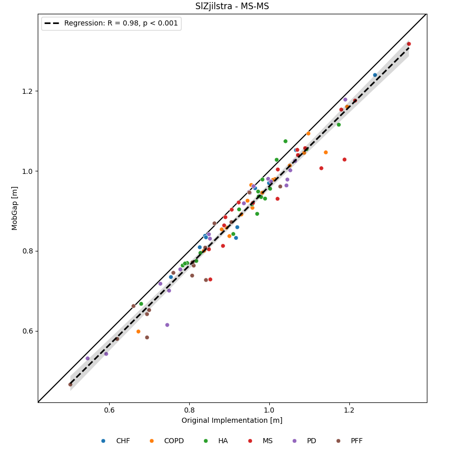
Below, we show the direct correlation between the results from the old and the new implementation. Each datapoint represents one participant.
def compare_scatter_plot(data):
    fig, ax = plt.subplots(figsize=(9, 9), constrained_layout=True)
    reformated_data = (
        data.pivot_table(
            values="wb__detected",
            index=("cohort", "participant_id"),
            columns="version",
        )
        .reset_index()
        .dropna(how="any")
    )

    min_max = calc_min_max_with_margin(
        reformated_data["Original Implementation"], reformated_data["MobGap"]
    )
    sns.scatterplot(
        reformated_data,
        x="Original Implementation",
        y="MobGap",
        hue="cohort",
        ax=ax,
    )
    plot_regline(
        reformated_data["Original Implementation"],
        reformated_data["MobGap"],
        ax=ax,
    )
    make_square(ax, min_max, draw_diagonal=True)
    move_legend_outside(fig, ax)
    ax.set_title(data.name)
    ax.set_xlabel("Original Implementation [m]")
    ax.set_ylabel("MobGap [m]")
    plt.show()


free_living_results.groupby("algo").apply(
    compare_scatter_plot, include_groups=False
)

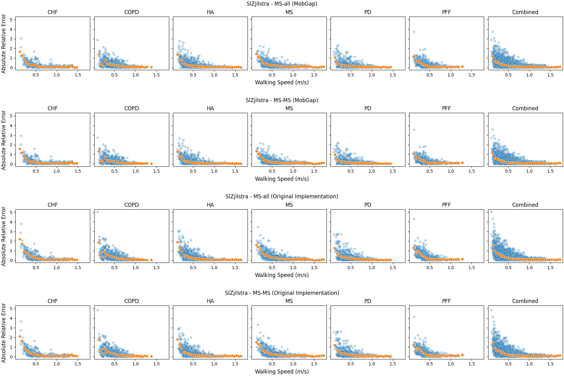
Speed dependency#
One important aspect of the algorithm performance is the dependency on the walking speed. Aka, how well do the algorithms perform at different walking speeds. For this we plot the absolute relative error against the walking speed of the reference data. For better granularity, we use the values per WB, instead of the aggregates per participant.
The overlayed dots represent the trend-line calculated by taking the median of the absolute relative error within bins of 0.05 m/s.
import numpy as np

wb_level_results = format_loaded_results(
    {
        v: loader.load_single_csv_file(
            k, "free_living", "raw_wb_level_values_with_errors.csv"
        )
        for k, v in algorithms.items()
    },
    free_living_index_cols,
)

# For plotting all participants at the end
combined = wb_level_results.copy()
combined["cohort"] = "Combined"
wb_level_results = pd.concat([wb_level_results, combined]).reset_index(
    drop=True
)

algo_names = wb_level_results["algo_with_version"].unique()
cohort_names = wb_level_results["cohort"].unique()

wb_level_results["cohort"] = pd.Categorical(
    wb_level_results["cohort"], categories=cohort_names, ordered=True
)
wb_level_results["algo_with_version"] = pd.Categorical(
    wb_level_results["algo_with_version"], categories=algo_names, ordered=True
)


fig = plt.figure(constrained_layout=True, figsize=(18, 3 * len(algo_names)))
subfigs = fig.subfigures(len(algo_names), 1, wspace=0.1, hspace=0.1)

min_max_x = calc_min_max_with_margin(wb_level_results["reference_ws"])
min_max_y = calc_min_max_with_margin(wb_level_results["abs_rel_error"])

for subfig, (algo, data) in zip(
    subfigs, wb_level_results.groupby("algo_with_version", observed=True)
):
    subfig.suptitle(algo)
    subfig.supxlabel("Walking Speed (m/s)")
    subfig.supylabel("Absolute Relative Error")
    axs = subfig.subplots(1, len(cohort_names), sharex=True, sharey=True)
    for ax, (cohort, cohort_data) in zip(
        axs, data.groupby("cohort", observed=True)
    ):
        sns.scatterplot(
            data=cohort_data,
            x="reference_ws",
            y="abs_rel_error",
            ax=ax,
            alpha=0.3,
        )

        bins = np.arange(0, cohort_data["reference_ws"].max() + 0.05, 0.05)
        cohort_data["speed_bin"] = pd.cut(
            cohort_data["reference_ws"], bins=bins
        )

        # Calculate bin centers for plotting
        cohort_data["bin_center"] = cohort_data["speed_bin"].apply(
            lambda x: x.mid
        )

        # Calculate medians per bin and cohort
        binned_data = (
            cohort_data.groupby("bin_center", observed=True)["abs_rel_error"]
            .median()
            .reset_index()
        )

        # Plot median lines
        sns.scatterplot(
            data=binned_data,
            x="bin_center",
            y="abs_rel_error",
            ax=ax,
        )
        ax.set_title(cohort)
        ax.set_xlabel(None)
        ax.set_ylabel(None)

        ax.set_xlim(*min_max_x)
        ax.set_ylim(*min_max_y)

fig.show()
  0%|                                               | 0.00/280k [00:00<?, ?B/s]
  0%|                                               | 0.00/280k [00:00<?, ?B/s]
100%|███████████████████████████████████████| 280k/280k [00:00<00:00, 1.23GB/s]

  0%|                                               | 0.00/281k [00:00<?, ?B/s]
  0%|                                               | 0.00/281k [00:00<?, ?B/s]
100%|███████████████████████████████████████| 281k/281k [00:00<00:00, 1.49GB/s]

  0%|                                               | 0.00/276k [00:00<?, ?B/s]
  0%|                                               | 0.00/276k [00:00<?, ?B/s]
100%|███████████████████████████████████████| 276k/276k [00:00<00:00, 1.46GB/s]

  0%|                                               | 0.00/277k [00:00<?, ?B/s]
  0%|                                               | 0.00/277k [00:00<?, ?B/s]
100%|███████████████████████████████████████| 277k/277k [00:00<00:00, 1.43GB/s]
Laboratory Comparison#
Every datapoint below is one trial of a test. Note, that each datapoint is weighted equally in the calculation of the performance metrics. This is a limitation of this simple approach, as the number of strides per trial and the complexity of the context can vary significantly. For a full picture, different groups of tests should be analyzed separately. The approach below should still provide a good overview to compare the algorithms.
fig, ax = plt.subplots()
sns.boxplot(data=lab_results, x="algo_with_version", y="wb__abs_error", ax=ax)
plt.xticks(rotation=45, ha="right")
fig.tight_layout()
fig.show()

perf_metrics_all = lab_results.pipe(
    multilevel_groupby_apply_merge,
    [
        (
            ["algo", "version"],
            partial(apply_aggregations, aggregations=custom_aggs),
        ),
        (
            ["algo"],
            partial(apply_transformations, transformations=stats_transform),
        ),
    ],
).pipe(format_tables)
perf_metrics_all.style.pipe(
    revalidation_table_styles,
    validation_thresholds,
    ["algo"],
)
Per Cohort#
The results below represent the average performance across all trails of all participants within a cohort.
fig, ax = plt.subplots()
sns.boxplot(
    data=lab_results,
    x="cohort",
    y="wb__abs_error",
    hue="algo_with_version",
    order=cohort_order,
    ax=ax,
)
fig.show()
perf_metrics_cohort = (
    lab_results.pipe(
        multilevel_groupby_apply_merge,
        [
            (
                ["cohort", "algo", "version"],
                partial(apply_aggregations, aggregations=custom_aggs),
            ),
            (
                ["cohort", "algo"],
                partial(apply_transformations, transformations=stats_transform),
            ),
        ],
    )
    .pipe(format_tables)
    .loc[cohort_order]
)
perf_metrics_cohort.style.pipe(
    revalidation_table_styles,
    validation_thresholds,
    ["cohort", "algo"],
)
Total running time of the script: (0 minutes 13.631 seconds)
Estimated memory usage: 86 MB