Note
Go to the end to download the full example code.
Cadence estimation#
The following provides an analysis and comparison of the Mobilise-D algorithm pipeline on the Mobilise-D Technical Validation Study (TVS) dataset for the estimation of cadence (free-living). In this example, we look into the performance of the Python implementation of the pipeline compared to the reference data. We also compare the actual performance to that obtained by the original Matlab-based implementation [1].
Note
If you are interested in how these results are calculated, head over to the processing page.
from typing import Optional
Below the list of pipelines that are compared is shown. Note, that we use “MobGap” to refer to the reimplemented python algorithms, and the “Original Implementation” to refer to the original Matlab-based implementation.
algorithms = {
    "Official_MobiliseD_Pipeline": ("Mobilise-D Pipeline", "MobGap"),
    "EScience_MobiliseD_Pipeline": (
        "Mobilise-D Pipeline",
        "Original Implementation",
    ),
}
The code below loads the data and prepares it for the analysis.
By default, the data will be downloaded from an online repository (and cached locally).
If you want to use a local copy of the data, you can set the MOBGAP_VALIDATION_DATA_PATH environment variable.
and the MOBGAP_VALIDATION_USE_LOCA_DATA to 1.
The file download will print a couple log information, which can usually be ignored.
You can also change the version parameter to load a different version of the data.
from pathlib import Path

import pandas as pd
from mobgap.data.validation_results import ValidationResultLoader
from mobgap.utils.misc import get_env_var


def format_loaded_results(
    values: dict[tuple[str, str], pd.DataFrame],
    index_cols: list[str],
    col_prefix_filter: Optional[str],
    convert_rel_error: bool = False,
) -> pd.DataFrame:
    formatted = (
        pd.concat(values, names=["algo", "version", *index_cols])
        .pipe(
            lambda df: (
                df.filter(like=col_prefix_filter) if col_prefix_filter else df
            )
        )
        .reset_index()
        .assign(
            algo_with_version=lambda df: (
                df["algo"] + " (" + df["version"] + ")"
            ),
            _combined="combined",
        )
    )

    if col_prefix_filter:
        formatted.columns = formatted.columns.str.removeprefix(
            col_prefix_filter
        )

    if convert_rel_error:
        rel_cols = [c for c in formatted.columns if "rel_error" in c]
        formatted[rel_cols] = formatted[rel_cols] * 100

    return formatted


local_data_path = (
    Path(get_env_var("MOBGAP_VALIDATION_DATA_PATH")) / "results"
    if int(get_env_var("MOBGAP_VALIDATION_USE_LOCAL_DATA", 0))
    else None
)
__RESULT_VERSION = "v1.2.0"
loader = ValidationResultLoader(
    "full_pipeline", result_path=local_data_path, version=__RESULT_VERSION
)

# Loading free-living data
free_living_index_cols = [
    "cohort",
    "participant_id",
    "time_measure",
    "recording",
    "recording_name",
    "recording_name_pretty",
]

_free_living_results = {  # Matched and aggregate/combined per-recording results for the 2.5 h free-living recordings
    v: loader.load_single_results(k, "free_living")
    for k, v in algorithms.items()
}

_free_living_results_raw = {  # Matched per-WB results for the 2.5 h free-living recordings
    v: loader.load_single_csv_file(k, "free_living", "raw_matched_errors.csv")
    for k, v in algorithms.items()
}
free_living_results_combined = format_loaded_results(
    _free_living_results,
    free_living_index_cols,
    "combined__",
    convert_rel_error=True,
)
free_living_results_matched = format_loaded_results(
    _free_living_results,
    free_living_index_cols,
    "matched__",
    convert_rel_error=True,
)
free_living_results_matched_raw = format_loaded_results(
    values=_free_living_results_raw,
    index_cols=free_living_index_cols,
    col_prefix_filter=None,
    convert_rel_error=True,
)

del _free_living_results, _free_living_results_raw

# Loading laboratory data
laboratory_index_cols = [
    "cohort",
    "participant_id",
    "time_measure",
    "test",
    "trial",
    "test_name",
    "test_name_pretty",
]

_laboratory_results = {  # Matched and aggregate/combined per-recording results for the laboratory recordings
    v: loader.load_single_results(k, "laboratory")
    for k, v in algorithms.items()
}

_laboratory_results_raw = {  # Matched per-WB results for the laboratory recordings
    v: loader.load_single_csv_file(k, "laboratory", "raw_matched_errors.csv")
    for k, v in algorithms.items()
}
laboratory_results_combined = format_loaded_results(
    _laboratory_results,
    laboratory_index_cols,
    "combined__",
    convert_rel_error=True,
)
laboratory_results_matched = format_loaded_results(
    _laboratory_results,
    laboratory_index_cols,
    "matched__",
    convert_rel_error=True,
)
laboratory_results_matched_raw = format_loaded_results(
    values=_laboratory_results_raw,
    index_cols=laboratory_index_cols,
    col_prefix_filter=None,
    convert_rel_error=True,
)

del _laboratory_results, _laboratory_results_raw
cohort_order = ["HA", "CHF", "COPD", "MS", "PD", "PFF"]
Performance metrics#
Below you can find the setup for all performance metrics that we will calculate.
We only use the single__ results for the comparison.
Note
For the evaluation of the full pipeline performance, two types of aggregation are performed, which will be described later on in the example.
from functools import partial

from mobgap.pipeline.evaluation import CustomErrorAggregations as A
from mobgap.utils.df_operations import (
    CustomOperation,
    apply_aggregations,
    apply_transformations,
    multilevel_groupby_apply_merge,
)
from mobgap.utils.tables import FormatTransformer as F
from mobgap.utils.tables import RevalidationInfo, revalidation_table_styles
from mobgap.utils.tables import StatsFunctions as S

custom_aggs_combined = [
    CustomOperation(
        identifier=None,
        function=A.n_datapoints,
        column_name=[("n_datapoints", "all")],
    ),
    ("cadence_spm__detected", ["mean", A.conf_intervals]),
    ("cadence_spm__reference", ["mean", A.conf_intervals]),
    ("cadence_spm__error", ["mean", A.loa]),
    ("cadence_spm__abs_error", ["mean", A.conf_intervals]),
    ("cadence_spm__rel_error", ["mean", A.conf_intervals]),
    ("cadence_spm__abs_rel_error", ["mean", A.conf_intervals]),
    CustomOperation(
        identifier=None,
        function=partial(
            A.icc,
            reference_col_name="cadence_spm__reference",
            detected_col_name="cadence_spm__detected",
            icc_type="icc2",
            # For the lab data, some trials have no results for the old algorithms.
            nan_policy="omit",
        ),
        column_name=[("icc", "all"), ("icc_ci", "all")],
    ),
]

custom_aggs_matched = [
    CustomOperation(
        identifier=None,
        function=lambda df_: df_["n_matched_wbs"].sum(),
        column_name=[("n_wbs_matched", "all")],
    ),
    *custom_aggs_combined,
]

stats_transform = [
    CustomOperation(
        identifier=None,
        function=partial(
            S.pairwise_tests,
            value_col=c,
            between="version",
            reference_group_key="Original Implementation",
        ),
        column_name=[("stats_metadata", c)],
    )
    for c in [
        "cadence_spm__abs_error",
        "cadence_spm__abs_rel_error",
    ]
]

format_transforms_combined = [
    CustomOperation(
        identifier=None,
        function=lambda df_: df_[("n_datapoints", "all")].astype(int),
        column_name="n_datapoints",
    ),
    *(
        CustomOperation(
            identifier=None,
            function=partial(
                F.value_with_metadata,
                value_col=("mean", c),
                other_columns={
                    "range": ("conf_intervals", c),
                    "stats_metadata": ("stats_metadata", c),
                },
            ),
            column_name=c,
        )
        for c in [
            "cadence_spm__reference",
            "cadence_spm__detected",
            "cadence_spm__abs_error",
            "cadence_spm__rel_error",
            "cadence_spm__abs_rel_error",
        ]
    ),
    CustomOperation(
        identifier=None,
        function=partial(
            F.value_with_metadata,
            value_col=("mean", "cadence_spm__error"),
            other_columns={"range": ("loa", "cadence_spm__error")},
        ),
        column_name="cadence_spm__error",
    ),
    CustomOperation(
        identifier=None,
        function=partial(
            F.value_with_metadata,
            value_col=("icc", "all"),
            other_columns={"range": ("icc_ci", "all")},
        ),
        column_name="icc",
    ),
]

format_transforms_matched = [
    CustomOperation(
        identifier=None,
        function=lambda df_: df_[("n_wbs_matched", "all")].astype(int),
        column_name="n_wbs_matched",
    ),
    *format_transforms_combined,
]


final_names_combined = {
    "n_datapoints": "# participants",
    "cadence_spm__detected": "WD mean and CI [steps/min]",
    "cadence_spm__reference": "INDIP mean and CI [steps/min]",
    "cadence_spm__error": "Bias and LoA [steps/min]",
    "cadence_spm__abs_error": "Abs. Error [steps/min]",
    "cadence_spm__rel_error": "Rel. Error [%]",
    "cadence_spm__abs_rel_error": "Abs. Rel. Error [%]",
    "icc": "ICC",
}

final_names_matched = {
    **final_names_combined,
    "n_wbs_matched": "# Matched WBs",
}

validation_thresholds = {
    "Abs. Error [steps/min]": RevalidationInfo(
        threshold=None, higher_is_better=False
    ),
    "Abs. Rel. Error [%]": RevalidationInfo(
        threshold=20, higher_is_better=False
    ),
    "ICC": RevalidationInfo(threshold=0.7, higher_is_better=True),
}


def format_tables_combined(df: pd.DataFrame) -> pd.DataFrame:
    return (
        df.pipe(apply_transformations, format_transforms_combined)
        .rename(columns=final_names_combined)
        .loc[:, list(final_names_combined.values())]
    )


def format_tables_matched(df: pd.DataFrame) -> pd.DataFrame:
    return (
        df.pipe(apply_transformations, format_transforms_matched)
        .rename(columns=final_names_matched)
        .loc[:, list(final_names_matched.values())]
    )
Free-living dataset#
Combined/Aggregated Evaluation#
To mimic actual use of wearable device where actual decisions are made on aggregated measures over a longer measurement period and not WB per WB, our primary comparison is based on the median gait metrics over the entire recording. We call this combined or aggregated evaluation. For this we combined all WBs for a datapoint by taking the median of the calculated cadence. These combined values were then compared between the systems.
Note
In the free-living dataset, each datapoint represents one 2.5h recording.
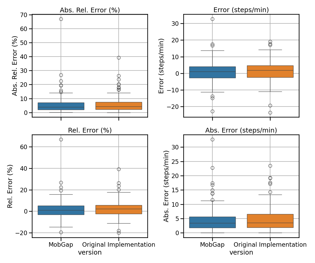
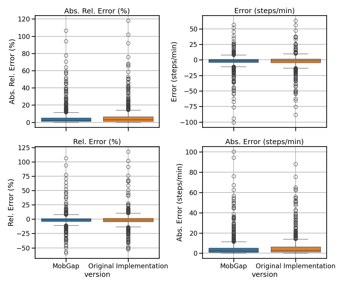
All results across all cohorts#
The results below represent the average performance across all participants independent of the cohort in terms of error, relative error, absolute error, and absolute relative error.
import matplotlib.pyplot as plt
import seaborn as sns

sns.set_context("talk")
metrics = {
    "abs_rel_error": "Abs. Rel. Error (%)",
    "error": "Error (steps/min)",
    "rel_error": "Rel. Error (%)",
    "abs_error": "Abs. Error (steps/min)",
}


def multi_metric_plot(data, metrics, nrows, ncols):
    fig, axs = plt.subplots(
        nrows, ncols, sharex=True, figsize=(ncols * 6, nrows * 4 + 2)
    )
    for ax, (metric, metric_label) in zip(axs.flatten(), metrics.items()):
        overall_df = data[["version", f"cadence_spm__{metric}"]].rename(
            columns={f"cadence_spm__{metric}": metric_label}
        )

        sns.boxplot(
            data=overall_df, x="version", hue="version", y=metric_label, ax=ax
        )

        ax.set_title(metric_label)
        ax.set_ylabel(metric_label)

        ax.tick_params(axis="both", which="major")
        ax.tick_params(axis="both", which="minor")

        ax.grid(True)

    plt.tight_layout()
    plt.show()


free_living_results_combined.pipe(multi_metric_plot, metrics, 2, 2)
free_living_combined_perf_metrics_all = free_living_results_combined.pipe(
    multilevel_groupby_apply_merge,
    [
        (
            ["algo", "version"],
            partial(apply_aggregations, aggregations=custom_aggs_combined),
        ),
        (
            ["algo"],
            partial(apply_transformations, transformations=stats_transform),
        ),
    ],
).pipe(format_tables_combined)
free_living_combined_perf_metrics_all.style.pipe(
    revalidation_table_styles,
    validation_thresholds,
    ["algo"],
)
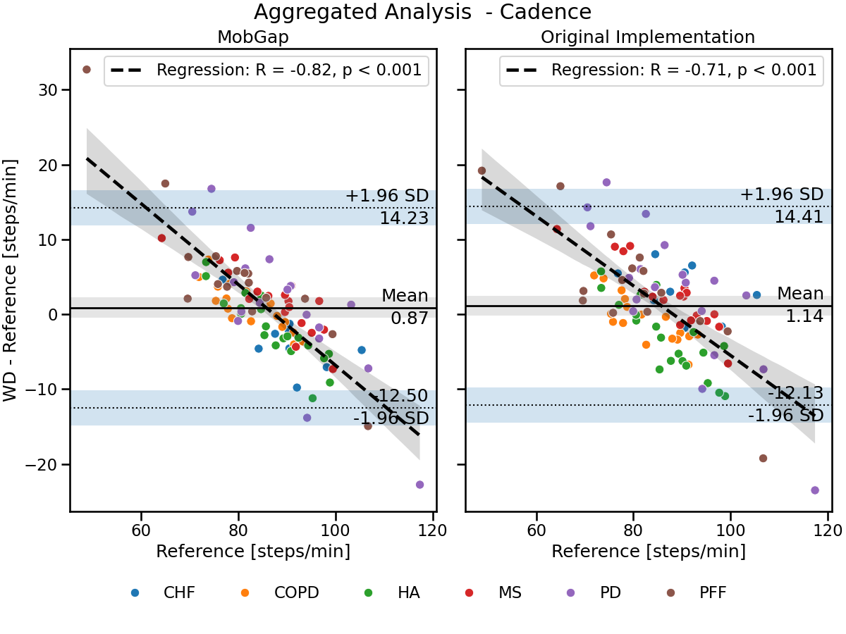
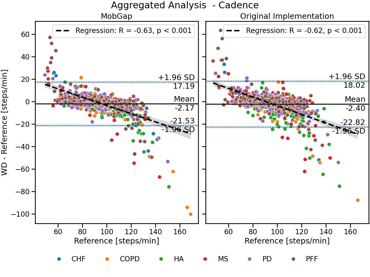
Residual plots
from mobgap.plotting import move_legend_outside, residual_plot


def combo_residual_plot(data, name=None):
    name = name or data.name
    fig, axs = plt.subplots(
        ncols=2,
        sharey=True,
        sharex=True,
        figsize=(12, 9),
        constrained_layout=True,
    )
    fig.suptitle(name)
    for (version, subdata), ax in zip(data.groupby("version"), axs):
        residual_plot(
            subdata,
            "cadence_spm__reference",
            "cadence_spm__detected",
            "cohort",
            "steps/min",
            ax=ax,
            legend=ax == axs[-1],
        )
        ax.set_title(version)
    move_legend_outside(fig, axs[-1])
    plt.show()


free_living_results_combined.query('algo == "Mobilise-D Pipeline"').pipe(
    combo_residual_plot, name="Aggregated Analysis  - Cadence"
)
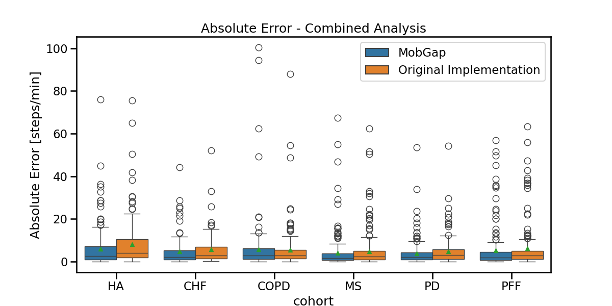
Per-cohort analysis#
The results below represent the average absolute error on cadence estimation across all participants within a cohort.
fig, ax = plt.subplots(figsize=(12, 6))
sns.boxplot(
    data=free_living_results_combined,
    x="cohort",
    y="cadence_spm__abs_error",
    hue="version",
    order=cohort_order,
    showmeans=True,
    ax=ax,
).legend().set_title(None)
ax.set_ylabel("Absolute Error [steps/min]")
ax.set_title("Absolute Error - Combined Analysis")
fig.show()

free_living_combined_perf_metrics_cohort = (
    free_living_results_combined.pipe(
        multilevel_groupby_apply_merge,
        [
            (
                ["cohort", "algo", "version"],
                partial(apply_aggregations, aggregations=custom_aggs_combined),
            ),
            (
                ["cohort", "algo"],
                partial(apply_transformations, transformations=stats_transform),
            ),
        ],
    )
    .pipe(format_tables_combined)
    .loc[cohort_order]
)
free_living_combined_perf_metrics_cohort.style.pipe(
    revalidation_table_styles,
    validation_thresholds,
    ["cohort", "algo"],
)
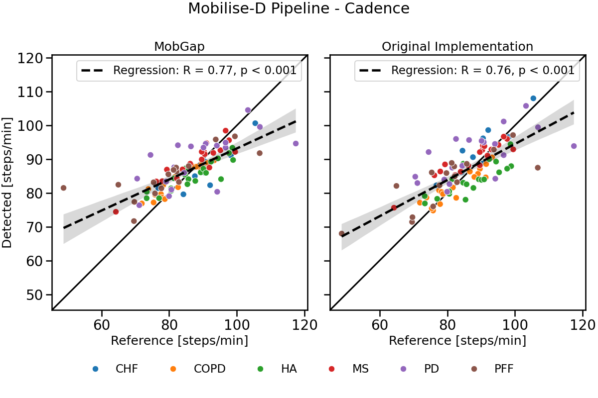
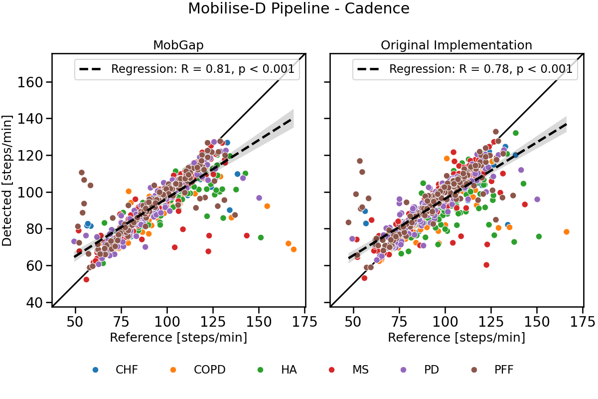
Scatter plot The results below represent the detected and reference values of cadence scattered across all participants within a cohort. Correlation factor, p-value and confidence intervals of the regression line are shown in the plot. Each datapoint represents one participant.
from mobgap.plotting import calc_min_max_with_margin, make_square, plot_regline


def combo_scatter_plot(data, name=None):
    name = name or data.name
    fig, axs = plt.subplots(
        ncols=2,
        sharey=True,
        sharex=True,
        figsize=(12, 8),
        constrained_layout=True,
    )
    fig.suptitle(name)

    min_max = calc_min_max_with_margin(
        data["cadence_spm__reference"],
        data["cadence_spm__detected"],
    )

    for (version, subdata), ax in zip(data.groupby("version"), axs):
        subdata = subdata[
            [
                "cadence_spm__reference",
                "cadence_spm__detected",
                "cohort",
            ]
        ].dropna(how="any")

        sns.scatterplot(
            subdata,
            x="cadence_spm__reference",
            y="cadence_spm__detected",
            hue="cohort",
            ax=ax,
            legend=ax == axs[-1],
        )

        plot_regline(
            subdata["cadence_spm__reference"],
            subdata["cadence_spm__detected"],
            ax=ax,
        )

        make_square(ax, min_max, draw_diagonal=True)

        ax.set_title(version)
        ax.set_xlabel("Reference [steps/min]")
        ax.set_ylabel("Detected [steps/min]")
        ax.tick_params(axis="both", labelsize=20)

    move_legend_outside(fig, axs[-1])

    plt.show()


free_living_results_combined.query('algo == "Mobilise-D Pipeline"').pipe(
    combo_scatter_plot, name="Mobilise-D Pipeline - Cadence"
)
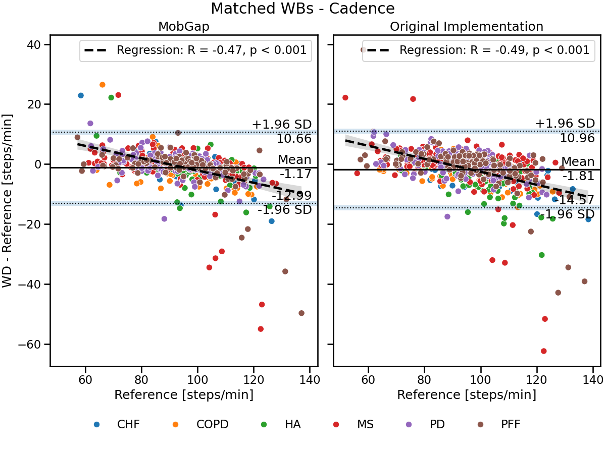
Matched/True Positive Evaluation#
The “Matched” Evaluation directly compares the performance of cadence estimation on only the WBs that were detected in both systems (true positives). WBs were included in the true positive analysis, if there was an overlap of more than 80% between WBs detected by the two systems (details about the selection of this threshold can be found in [1]). The threshold of 80% was selected as a trade-off to allow us: (i) to consider as much as possible a like-for-like comparison between selected WBs (INDIP vs. wearable device), and at the same time (ii) to include the minimum number of WBs to ensure sufficient statistical power for the analyses (i.e., at least 101 walking bouts for each cohort). This target was based upon the number of WBs rather than a percentage of total walking bouts that would allow us to meet criteria established by statistical experts for robust statistical analysis after sample-size re-evaluation (total WB number > 101 corresponding to ICC > 0.7 and a CI = 0.2).
Note
compared to the results published in [1], the primary analysis on the matched results is performed on the average performance metrics across all matched WBs per recording/per participant. The original publication considered the average performance metrics across all matched WBs without additional aggregation.
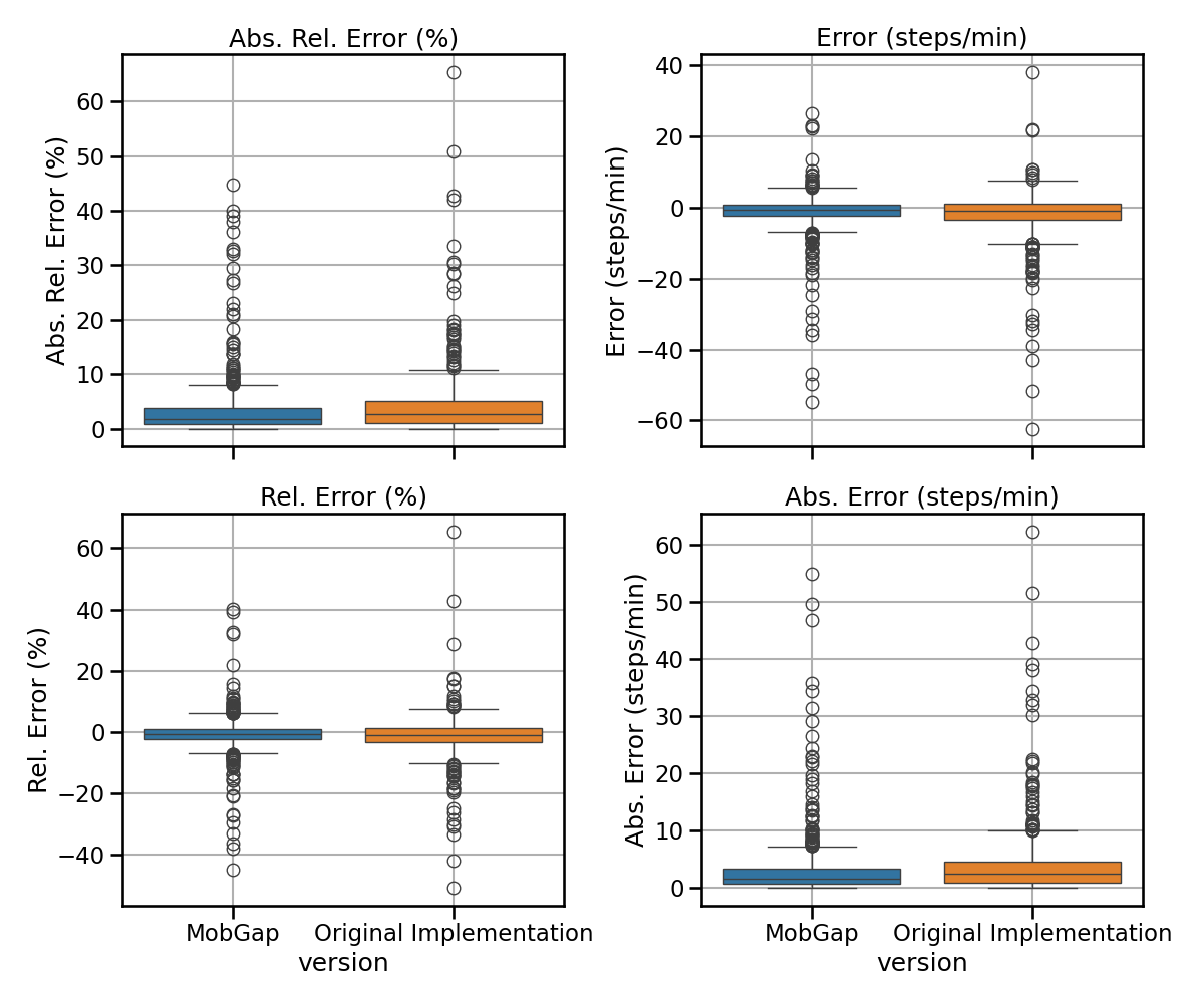
Results across all cohorts#
The results below represent the average performance across all participants independent of the cohort in terms of error, relative error, absolute error, and absolute relative error.
free_living_results_matched.pipe(multi_metric_plot, metrics, 2, 2)
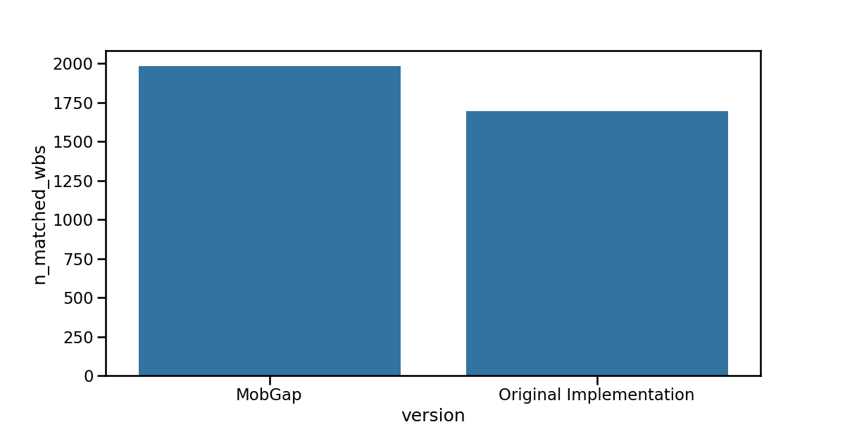
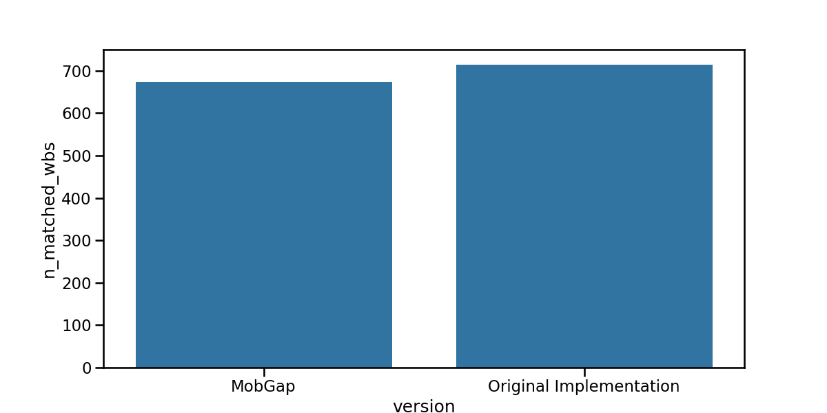
As each pipeline version produces different WB’s, it is important to compare the number of matched WBs to put all other metrics into perspective.
fig, ax = plt.subplots(figsize=(12, 6))
sns.barplot(
    data=free_living_results_matched.groupby(["version"])["n_matched_wbs"]
    .sum()
    .reset_index(),
    x="version",
    y="n_matched_wbs",
    ax=ax,
)
fig.show()
free_living_matched_perf_metrics_all = free_living_results_matched.pipe(
    multilevel_groupby_apply_merge,
    [
        (
            ["algo", "version"],
            partial(apply_aggregations, aggregations=custom_aggs_matched),
        ),
        (
            ["algo"],
            partial(apply_transformations, transformations=stats_transform),
        ),
    ],
).pipe(format_tables_matched)

free_living_matched_perf_metrics_all.style.pipe(
    revalidation_table_styles,
    validation_thresholds,
    ["algo"],
)
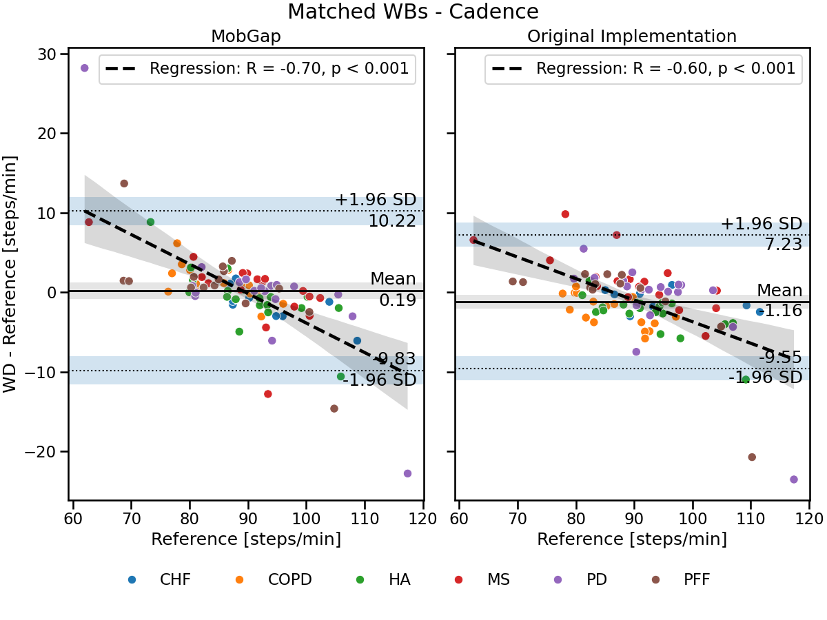
Residual plot
free_living_results_matched.query('algo == "Mobilise-D Pipeline"').pipe(
    combo_residual_plot, name="Matched WBs - Cadence"
)
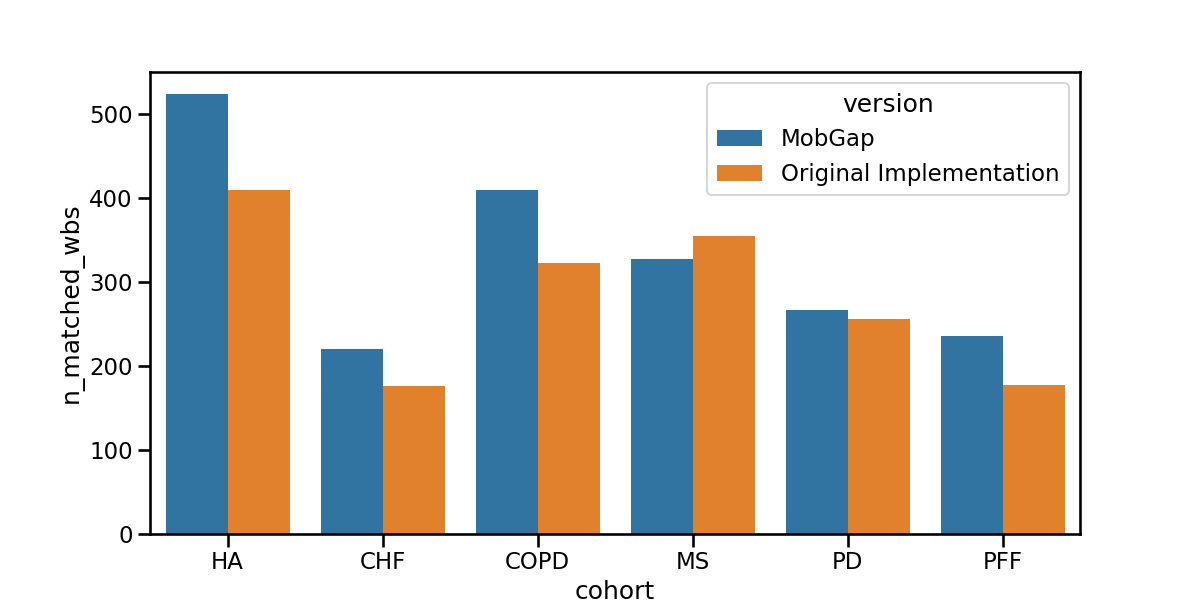
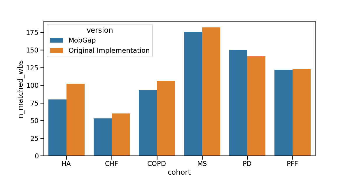
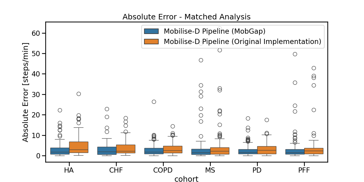
Per-cohort analysis#
Boxplot The results below represent the average absolute error on cadence estimation across all participants within a cohort.
fig, ax = plt.subplots(figsize=(12, 6))
sns.barplot(
    data=free_living_results_matched.groupby(["version", "cohort"])[
        "n_matched_wbs"
    ]
    .sum()
    .reset_index(),
    hue="version",
    y="n_matched_wbs",
    x="cohort",
    order=cohort_order,
    ax=ax,
)
fig.show()
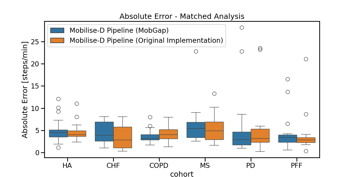
fig, ax = plt.subplots(figsize=(12, 6))
sns.boxplot(
    data=free_living_results_matched,
    x="cohort",
    y="cadence_spm__abs_error",
    hue="algo_with_version",
    order=cohort_order,
    ax=ax,
).legend().set_title(None)
ax.set_ylabel("Absolute Error [steps/min]")
ax.set_title("Absolute Error - Matched Analysis")
fig.show()
Processing the per-cohort performance table
free_living_matched_perf_metrics_cohort = (
    free_living_results_matched.pipe(
        multilevel_groupby_apply_merge,
        [
            (
                ["cohort", "algo", "version"],
                partial(apply_aggregations, aggregations=custom_aggs_matched),
            ),
            (
                ["cohort", "algo"],
                partial(apply_transformations, transformations=stats_transform),
            ),
        ],
    )
    .pipe(format_tables_matched)
    .loc[cohort_order]
)

free_living_matched_perf_metrics_cohort.style.pipe(
    revalidation_table_styles,
    validation_thresholds,
    ["cohort", "algo"],
)
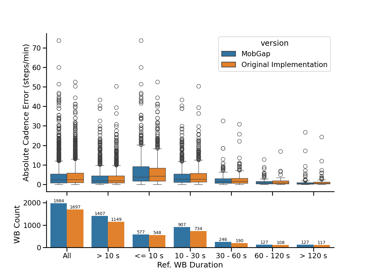
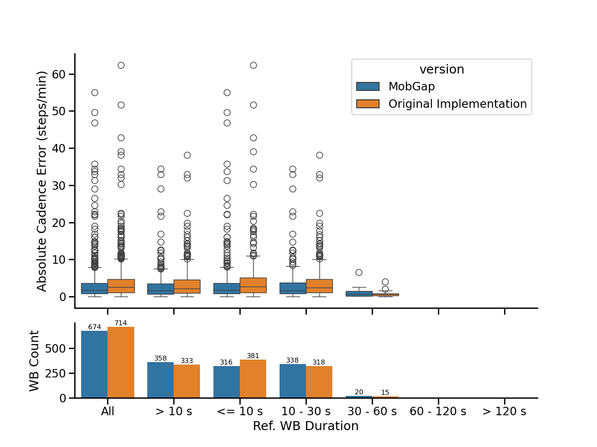
Deep dive investigation: Do errors depend on WB duration or walking speed?#
Effect of WB duration#
We investigate the dependency of the absolute cadence error of all true-positive WBs from the real-world recording on the WB duration reported by the reference system. In the top, WB errors are grouped by various duration bouts. In the bottom the number of bouts within each duration group is visualized.
import numpy as np
from mobgap.utils.df_operations import cut_into_overlapping_bins


def plot_wb_duration_analysis(df):
    """Generates a single figure with:
    - First row: Two side-by-side boxplot for "new" and "old" cases.
    - Second row: A grouped bar chart comparing WB counts for "new" and "old" cases.

    df: DataFrame containing 'version' column with values 'new' or 'old' to distinguish data
    """
    fig, axs = plt.subplot_mosaic(
        [["v"], ["v"], ["v"], ["n"]], sharex=True, figsize=(12, 9)
    )
    # Compute WB durations in seconds
    df_with_durations = df.assign(
        duration_s=lambda df_: (
            (df_["end__reference"] - df_["start__reference"]) / 100
        )
    )

    bins = {
        "All": (-np.inf, np.inf),
        "> 10 s": (10, np.inf),
        "<= 10 s": (0, 10),
        "10 - 30 s": (10, 30),
        "30 - 60 s": (30, 60),
        "60 - 120 s": (60, 120),
        "> 120 s": (120, np.inf),
    }

    binned_df = cut_into_overlapping_bins(
        df_with_durations, "duration_s", bins
    ).reset_index()
    n = sns.countplot(
        data=binned_df, x="bin", hue="version", ax=axs["n"], legend=False
    )
    for container in n.containers:
        n.bar_label(container, size=10)

    sns.boxplot(
        data=binned_df,
        x="bin",
        y="cadence_spm__abs_error",
        hue="version",
        ax=axs["v"],
    )
    sns.despine(fig)

    axs["v"].set_ylabel("Absolute Cadence Error (steps/min)")
    axs["n"].set_ylabel("WB Count")
    axs["n"].set_xlabel("Ref. WB Duration")
    fig.show()


free_living_results_matched_raw.query("algo == 'Mobilise-D Pipeline'").pipe(
    plot_wb_duration_analysis
)
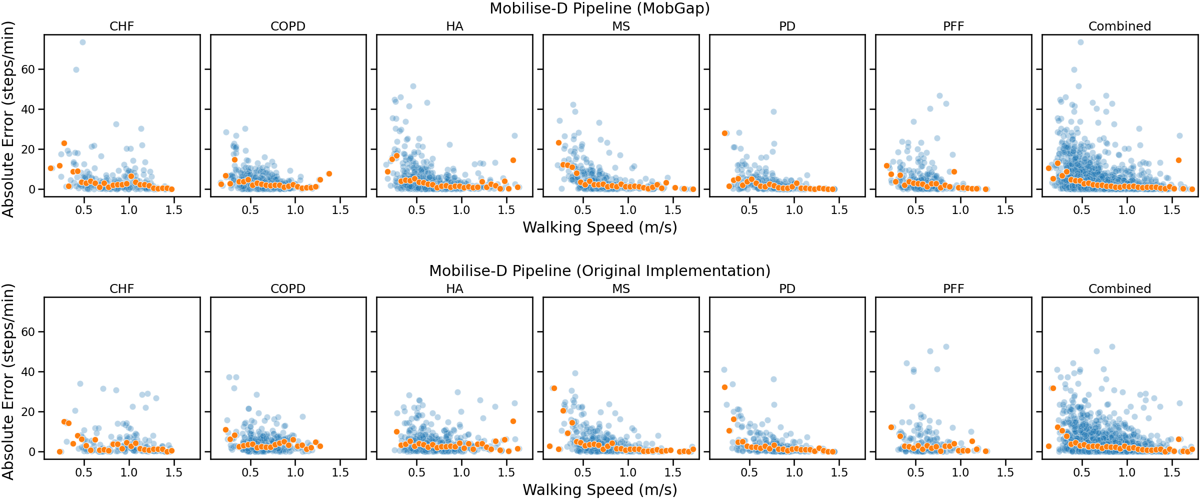
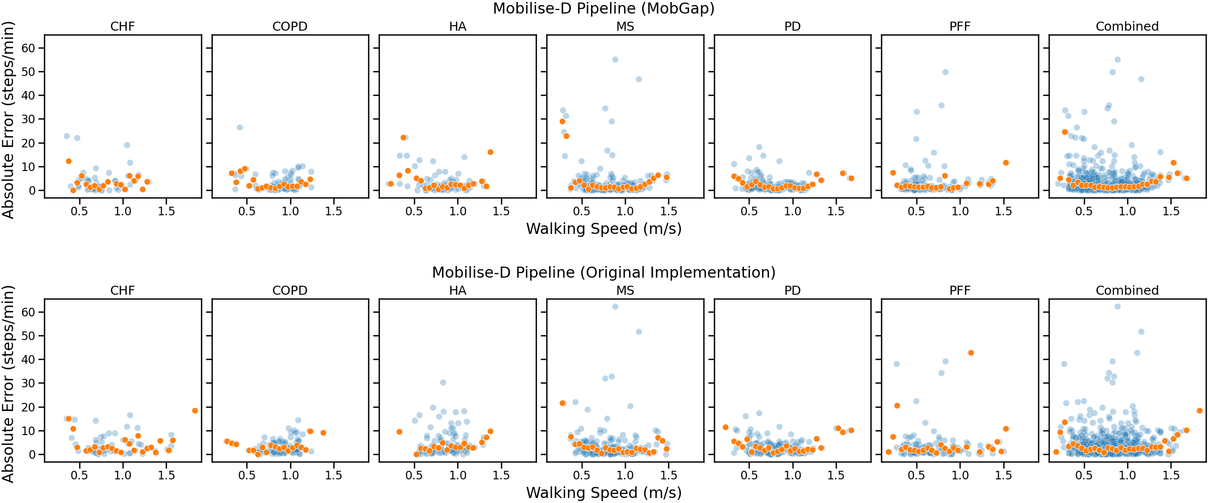
Effect of walking speed on error#
One important aspect of the algorithm performance is the dependency on the cadence. Aka, how well do the algorithms perform at different walking speeds. For this we plot the absolute error against the cadence of the reference data. For better granularity, we use the values per WB, instead of the aggregates per participant. The overlayed dots represent the trend-line calculated by taking the median of the absolute error within bins of 0.05 m/s.
# For plotting all participants at the end
free_living_combined = free_living_results_matched_raw.copy()
free_living_combined["cohort"] = "Combined"
ws_level_results = pd.concat(
    [free_living_results_matched_raw, free_living_combined]
).reset_index(drop=True)

algo_names = ws_level_results["algo_with_version"].unique()
cohort_names = ws_level_results["cohort"].unique()

ws_level_results["cohort"] = pd.Categorical(
    ws_level_results["cohort"], categories=cohort_names, ordered=True
)
ws_level_results["algo_with_version"] = pd.Categorical(
    ws_level_results["algo_with_version"], categories=algo_names, ordered=True
)

# Create the figure with subplots
fig = plt.figure(constrained_layout=True, figsize=(24, 5 * len(algo_names)))
subfigs = fig.subfigures(len(algo_names), 1, wspace=0.1, hspace=0.1)

# Define the min and max limits for x and y axes
min_max_x = calc_min_max_with_margin(
    ws_level_results["walking_speed_mps__reference"]
)
min_max_y = calc_min_max_with_margin(ws_level_results["cadence_spm__abs_error"])

# Plotting each algorithm version
for subfig, (algo, data) in zip(
    subfigs, ws_level_results.groupby("algo_with_version", observed=True)
):
    subfig.suptitle(algo)
    subfig.supxlabel("Walking Speed (m/s)")
    subfig.supylabel("Absolute Error (steps/min)")

    # Create subplots for each cohort
    axs = subfig.subplots(1, len(cohort_names), sharex=True, sharey=True)

    for ax, (cohort, cohort_data) in zip(
        axs, data.groupby("cohort", observed=True)
    ):
        # Scatter plot for the cohort data
        sns.scatterplot(
            data=cohort_data,
            x="walking_speed_mps__reference",  # Reference walking speed
            y="cadence_spm__abs_error",  # Absolute error
            ax=ax,
            alpha=0.3,
        )

        # Define bins for walking speed
        bins = np.arange(
            0, cohort_data["walking_speed_mps__reference"].max() + 0.05, 0.05
        )
        cohort_data["speed_bin"] = pd.cut(
            cohort_data["walking_speed_mps__reference"], bins=bins
        )

        # Calculate bin centers
        cohort_data["bin_center"] = cohort_data["speed_bin"].apply(
            lambda x: x.mid
        )

        # Calculate median error per bin and cohort
        binned_data = (
            cohort_data.groupby("bin_center", observed=True)[
                "cadence_spm__abs_error"
            ]
            .median()
            .reset_index()
        )

        # Plot the median lines for each bin
        sns.scatterplot(
            data=binned_data,
            x="bin_center",
            y="cadence_spm__abs_error",  # Median error
            ax=ax,
        )

        ax.set_title(cohort)
        ax.set_xlabel(None)
        ax.set_ylabel(None)

        # Set axis limits
        ax.set_xlim(*min_max_x)
        ax.set_ylim(*min_max_y)

fig.show()
Laboratory dataset#
Combined/Aggregated Evaluation#
To mimic actual use of wearable device where actual decisions are made on aggregated measures over a longer measurement period and not WB per WB, our primary comparison is based on the median gait metrics over the entire recording. We call this combined or aggregated evaluation. For this we combined all WBs for a datapoint by taking the median of the calculated cadence. These combined values were then compared between the systems.
Note
In the laboratory dataset, each datapoint represents one trial.
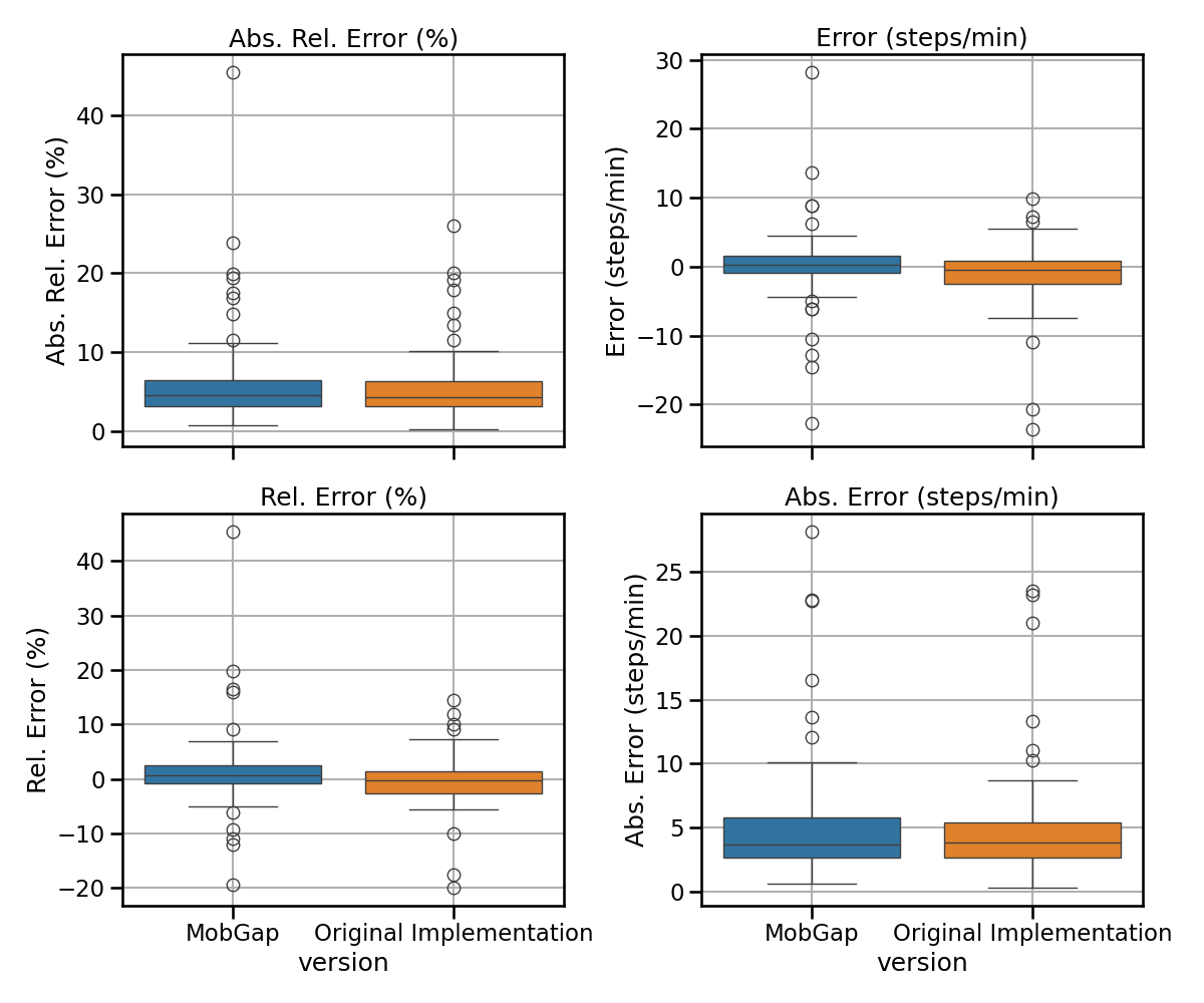
All results across all cohorts#
The results below represent the average performance across all participants independent of the cohort in terms of error, relative error, absolute error, and absolute relative error.
import matplotlib.pyplot as plt
import seaborn as sns

sns.set_context("talk")
metrics = {
    "abs_rel_error": "Abs. Rel. Error (%)",
    "error": "Error (steps/min)",
    "rel_error": "Rel. Error (%)",
    "abs_error": "Abs. Error (steps/min)",
}


def multi_metric_plot(data, metrics, nrows, ncols):
    fig, axs = plt.subplots(
        nrows, ncols, sharex=True, figsize=(ncols * 6, nrows * 4 + 2)
    )
    for ax, (metric, metric_label) in zip(axs.flatten(), metrics.items()):
        overall_df = data[["version", f"cadence_spm__{metric}"]].rename(
            columns={f"cadence_spm__{metric}": metric_label}
        )

        sns.boxplot(
            data=overall_df, x="version", hue="version", y=metric_label, ax=ax
        )

        ax.set_title(metric_label)
        ax.set_ylabel(metric_label)

        ax.tick_params(axis="both", which="major")
        ax.tick_params(axis="both", which="minor")

        ax.grid(True)

    plt.tight_layout()
    plt.show()


laboratory_results_combined.pipe(multi_metric_plot, metrics, 2, 2)
laboratory_combined_perf_metrics_all = laboratory_results_combined.pipe(
    multilevel_groupby_apply_merge,
    [
        (
            ["algo", "version"],
            partial(apply_aggregations, aggregations=custom_aggs_combined),
        ),
        (
            ["algo"],
            partial(apply_transformations, transformations=stats_transform),
        ),
    ],
).pipe(format_tables_combined)

laboratory_combined_perf_metrics_all.style.pipe(
    revalidation_table_styles,
    validation_thresholds,
    ["algo"],
)
Residual plots
def combo_residual_plot(data, name=None):
    name = name or data.name
    fig, axs = plt.subplots(
        ncols=2,
        sharey=True,
        sharex=True,
        figsize=(12, 9),
        constrained_layout=True,
    )
    fig.suptitle(name)
    for (version, subdata), ax in zip(data.groupby("version"), axs):
        residual_plot(
            subdata,
            "cadence_spm__reference",
            "cadence_spm__detected",
            "cohort",
            "steps/min",
            ax=ax,
            legend=ax == axs[-1],
        )
        ax.set_title(version)
    move_legend_outside(fig, axs[-1])
    plt.show()


laboratory_results_combined.query('algo == "Mobilise-D Pipeline"').pipe(
    combo_residual_plot, name="Aggregated Analysis  - Cadence"
)
Per-cohort analysis#
The results below represent the average absolute error on cadence estimation across all participants within a cohort.
fig, ax = plt.subplots(figsize=(12, 6))
sns.boxplot(
    data=laboratory_results_combined,
    x="cohort",
    y="cadence_spm__abs_error",
    hue="version",
    order=cohort_order,
    showmeans=True,
    ax=ax,
).legend().set_title(None)
ax.set_ylabel("Absolute Error [steps/min]")
ax.set_title("Absolute Error - Combined Analysis")
fig.show()
laboratory_combined_perf_metrics_cohort = (
    laboratory_results_combined.pipe(
        multilevel_groupby_apply_merge,
        [
            (
                ["cohort", "algo", "version"],
                partial(apply_aggregations, aggregations=custom_aggs_combined),
            ),
            (
                ["cohort", "algo"],
                partial(apply_transformations, transformations=stats_transform),
            ),
        ],
    )
    .pipe(format_tables_combined)
    .loc[cohort_order]
)
laboratory_combined_perf_metrics_cohort.style.pipe(
    revalidation_table_styles,
    validation_thresholds,
    ["cohort", "algo"],
)
Scatter plot The results below represent the detected and reference values of cadence scattered across all participants within a cohort. Correlation factor, p-value and confidence intervals of the regression line are shown in the plot. Each datapoint represents one participant.
from mobgap.plotting import calc_min_max_with_margin


def combo_scatter_plot(data, name=None):
    name = name or data.name
    fig, axs = plt.subplots(
        ncols=2,
        sharey=True,
        sharex=True,
        figsize=(12, 8),
        constrained_layout=True,
    )
    fig.suptitle(name)

    min_max = calc_min_max_with_margin(
        data["cadence_spm__reference"],
        data["cadence_spm__detected"],
    )

    for (version, subdata), ax in zip(data.groupby("version"), axs):
        subdata = subdata[
            [
                "cadence_spm__reference",
                "cadence_spm__detected",
                "cohort",
            ]
        ].dropna(how="any")

        sns.scatterplot(
            subdata,
            x="cadence_spm__reference",
            y="cadence_spm__detected",
            hue="cohort",
            ax=ax,
            legend=ax == axs[-1],
        )

        plot_regline(
            subdata["cadence_spm__reference"],
            subdata["cadence_spm__detected"],
            ax=ax,
        )

        make_square(ax, min_max, draw_diagonal=True)

        ax.set_title(version)
        ax.set_xlabel("Reference [steps/min]")
        ax.set_ylabel("Detected [steps/min]")
        ax.tick_params(axis="both", labelsize=20)

    move_legend_outside(fig, axs[-1])

    plt.show()


laboratory_results_combined.query('algo == "Mobilise-D Pipeline"').pipe(
    combo_scatter_plot, name="Mobilise-D Pipeline - Cadence"
)
Matched/True Positive Evaluation#
The “Matched” Evaluation directly compares the performance of cadence estimation on only the WBs that were detected in both systems (true positives). WBs were included in the true positive analysis, if there was an overlap of more than 80% between WBs detected by the two systems (details about the selection of this threshold can be found in [1]). The threshold of 80% was selected as a trade-off to allow us: (i) to consider as much as possible a like-for-like comparison between selected WBs (INDIP vs. wearable device), and at the same time (ii) to include the minimum number of WBs to ensure sufficient statistical power for the analyses (i.e., at least 101 walking bouts for each cohort). This target was based upon the number of WBs rather than a percentage of total walking bouts that would allow us to meet criteria established by statistical experts for robust statistical analysis after sample-size re-evaluation (total WB number > 101 corresponding to ICC > 0.7 and a CI = 0.2).
Note
compared to the results published in [1], the primary analysis on the matched results is performed on the average performance metrics across all matched WBs per trial. The original publication considered the average performance metrics across all matched WBs without additional aggregation.
Results across all cohorts#
The results below represent the average performance across all participants independent of the cohort in terms of error, relative error, absolute error, and absolute relative error.
laboratory_results_matched.pipe(multi_metric_plot, metrics, 2, 2)
As each pipeline version produces different WB’s, it is important to compare the number of matched WBs to put all other metrics into perspective.
fig, ax = plt.subplots(figsize=(12, 6))
sns.barplot(
    data=laboratory_results_matched.groupby(["version"])["n_matched_wbs"]
    .sum()
    .reset_index(),
    x="version",
    y="n_matched_wbs",
    ax=ax,
)
fig.show()
laboratory_matched_perf_metrics_all = laboratory_results_matched.pipe(
    multilevel_groupby_apply_merge,
    [
        (
            ["algo", "version"],
            partial(apply_aggregations, aggregations=custom_aggs_matched),
        ),
        (
            ["algo"],
            partial(apply_transformations, transformations=stats_transform),
        ),
    ],
).pipe(format_tables_matched)

laboratory_matched_perf_metrics_all.style.pipe(
    revalidation_table_styles,
    validation_thresholds,
    ["algo"],
)
Residual plot
laboratory_results_matched.query('algo == "Mobilise-D Pipeline"').pipe(
    combo_residual_plot, name="Matched WBs - Cadence"
)
Per-cohort analysis#
Boxplot The results below represent the average absolute error on cadence estimation across all participants within a cohort.
fig, ax = plt.subplots(figsize=(12, 6))
sns.barplot(
    data=laboratory_results_matched.groupby(["version", "cohort"])[
        "n_matched_wbs"
    ]
    .sum()
    .reset_index(),
    hue="version",
    y="n_matched_wbs",
    x="cohort",
    order=cohort_order,
    ax=ax,
)
fig.show()
fig, ax = plt.subplots(figsize=(12, 6))
sns.boxplot(
    data=laboratory_results_matched,
    x="cohort",
    y="cadence_spm__abs_error",
    hue="algo_with_version",
    order=cohort_order,
    ax=ax,
).legend().set_title(None)
ax.set_ylabel("Absolute Error [steps/min]")
ax.set_title("Absolute Error - Matched Analysis")
fig.show()
Processing the per-cohort performance table
laboratory_matched_perf_metrics_cohort = (
    laboratory_results_matched.pipe(
        multilevel_groupby_apply_merge,
        [
            (
                ["cohort", "algo", "version"],
                partial(apply_aggregations, aggregations=custom_aggs_matched),
            ),
            (
                ["cohort", "algo"],
                partial(apply_transformations, transformations=stats_transform),
            ),
        ],
    )
    .pipe(format_tables_matched)
    .loc[cohort_order]
)

laboratory_matched_perf_metrics_cohort.style.pipe(
    revalidation_table_styles,
    validation_thresholds,
    ["cohort", "algo"],
)
Deep dive investigation: Do errors depend on WB duration or walking speed?#
Effect of WB duration#
We investigate the dependency of the absolute cadence error of all true-positive WBs from the real-world recording on the WB duration reported by the reference system. In the top, WB errors are grouped by various duration bouts. In the bottom the number of bouts within each duration group is visualized.
import numpy as np


def plot_wb_duration_analysis(df):
    """Generates a single figure with:
    - First row: Two side-by-side boxplot for "new" and "old" cases.
    - Second row: A grouped bar chart comparing WB counts for "new" and "old" cases.

    df: DataFrame containing 'version' column with values 'new' or 'old' to distinguish data
    """
    fig, axs = plt.subplot_mosaic(
        [["v"], ["v"], ["v"], ["n"]], sharex=True, figsize=(12, 9)
    )
    # Compute WB durations in seconds
    df_with_durations = df.assign(
        duration_s=lambda df_: (
            (df_["end__reference"] - df_["start__reference"]) / 100
        )
    )

    bins = {
        "All": (-np.inf, np.inf),
        "> 10 s": (10, np.inf),
        "<= 10 s": (0, 10),
        "10 - 30 s": (10, 30),
        "30 - 60 s": (30, 60),
        "60 - 120 s": (60, 120),
        "> 120 s": (120, np.inf),
    }

    binned_df = cut_into_overlapping_bins(
        df_with_durations, "duration_s", bins
    ).reset_index()
    n = sns.countplot(
        data=binned_df, x="bin", hue="version", ax=axs["n"], legend=False
    )
    for container in n.containers:
        n.bar_label(container, size=10)

    sns.boxplot(
        data=binned_df,
        x="bin",
        y="cadence_spm__abs_error",
        hue="version",
        ax=axs["v"],
    )
    sns.despine(fig)

    axs["v"].set_ylabel("Absolute Cadence Error (steps/min)")
    axs["n"].set_ylabel("WB Count")
    axs["n"].set_xlabel("Ref. WB Duration")
    fig.show()


laboratory_results_matched_raw.query("algo == 'Mobilise-D Pipeline'").pipe(
    plot_wb_duration_analysis
)
Effect of walking speed on error#
One important aspect of the algorithm performance is the dependency on the cadence. Aka, how well do the algorithms perform at different walking speeds. For this we plot the absolute error against the cadence of the reference data. For better granularity, we use the values per WB, instead of the aggregates per participant. The overlayed dots represent the trend-line calculated by taking the median of the absolute error within bins of 0.05 m/s.
# For plotting all participants at the end
laboratory_combined = laboratory_results_matched_raw.copy()
laboratory_combined["cohort"] = "Combined"
ws_level_results = pd.concat(
    [laboratory_results_matched_raw, laboratory_combined]
).reset_index(drop=True)

algo_names = ws_level_results["algo_with_version"].unique()
cohort_names = ws_level_results["cohort"].unique()

ws_level_results["cohort"] = pd.Categorical(
    ws_level_results["cohort"], categories=cohort_names, ordered=True
)
ws_level_results["algo_with_version"] = pd.Categorical(
    ws_level_results["algo_with_version"], categories=algo_names, ordered=True
)

# Create the figure with subplots
fig = plt.figure(constrained_layout=True, figsize=(24, 5 * len(algo_names)))
subfigs = fig.subfigures(len(algo_names), 1, wspace=0.1, hspace=0.1)

# Define the min and max limits for x and y axes
min_max_x = calc_min_max_with_margin(
    ws_level_results["walking_speed_mps__reference"]
)
min_max_y = calc_min_max_with_margin(ws_level_results["cadence_spm__abs_error"])

# Plotting each algorithm version
for subfig, (algo, data) in zip(
    subfigs, ws_level_results.groupby("algo_with_version", observed=True)
):
    subfig.suptitle(algo)
    subfig.supxlabel("Walking Speed (m/s)")
    subfig.supylabel("Absolute Error (steps/min)")

    # Create subplots for each cohort
    axs = subfig.subplots(1, len(cohort_names), sharex=True, sharey=True)

    for ax, (cohort, cohort_data) in zip(
        axs, data.groupby("cohort", observed=True)
    ):
        # Scatter plot for the cohort data
        sns.scatterplot(
            data=cohort_data,
            x="walking_speed_mps__reference",  # Reference walking speed
            y="cadence_spm__abs_error",  # Absolute error
            ax=ax,
            alpha=0.3,
        )

        # Define bins for walking speed
        bins = np.arange(
            0, cohort_data["walking_speed_mps__reference"].max() + 0.05, 0.05
        )
        cohort_data["speed_bin"] = pd.cut(
            cohort_data["walking_speed_mps__reference"], bins=bins
        )

        # Calculate bin centers
        cohort_data["bin_center"] = cohort_data["speed_bin"].apply(
            lambda x: x.mid
        )

        # Calculate median error per bin and cohort
        binned_data = (
            cohort_data.groupby("bin_center", observed=True)[
                "cadence_spm__abs_error"
            ]
            .median()
            .reset_index()
        )

        # Plot the median lines for each bin
        sns.scatterplot(
            data=binned_data,
            x="bin_center",
            y="cadence_spm__abs_error",  # Median error
            ax=ax,
        )

        ax.set_title(cohort)
        ax.set_xlabel(None)
        ax.set_ylabel(None)

        # Set axis limits
        ax.set_xlim(*min_max_x)
        ax.set_ylim(*min_max_y)

fig.show()
Total running time of the script: (0 minutes 21.410 seconds)
Estimated memory usage: 91 MB