Note
Go to the end to download the full example code.
Performance of the gait sequences algorithm on the TVS dataset#
The following provides an analysis and comparison of the GSD performance on the TVS dataset (lab and free-living). We look into the actual performance of the algorithms compared to the reference data and compare these results with the performance of the original matlab algorithm.
Note
If you are interested in how these results are calculated, head over to the processing page.
We focus on the single_results (aka the performance per trail) and will aggregate it over multiple levels.
Below are the list of algorithms that we will compare.
Note, that we use the prefix “MobGap” to refer to the reimplemented python algorithms and “Original Implementation”
to refer to the original matlab algorithms.
In case of the GsdIluz algorithm, we also have two reimplemented versions.
The version MobGap uses a slightly modified peak detection algorithm, while the version MobGap (original peak)
tries to emulate the original peak detection algorithm as closely as possible.
algorithms = {
    "GsdIonescu": ("GsdIonescu", "MobGap"),
    "GsdAdaptiveIonescu": ("GsdAdaptiveIonescu", "MobGap"),
    "GsdIluz": ("GsdIluz", "MobGap"),
    "GsdIluz_orig_peak": ("GsdIluz", "MobGap (original peak)"),
}
# We only load the matlab algorithms that were also reimplemented
algorithms.update(
    {
        "matlab_EPFL_V1-improved_th": ("GsdIonescu", "Original Implementation"),
        "matlab_EPFL_V2-original": (
            "GsdAdaptiveIonescu",
            "Original Implementation",
        ),
        "matlab_TA_Iluz-original": ("GsdIluz", "Original Implementation"),
    }
)
The code below loads the data and prepares it for the analysis.
By default, the data will be downloaded from an online repository (and cached locally).
If you want to use a local copy of the data, you can set the MOBGAP_VALIDATION_DATA_PATH environment variable.
and the MOBGAP_VALIDATION_USE_LOCA_DATA to 1.
The file download will print a couple log information, which can usually be ignored.
You can also change the version parameter to load a different version of the data.
from pathlib import Path

import pandas as pd
from mobgap.data.validation_results import ValidationResultLoader
from mobgap.utils.misc import get_env_var

local_data_path = (
    Path(get_env_var("MOBGAP_VALIDATION_DATA_PATH")) / "results"
    if int(get_env_var("MOBGAP_VALIDATION_USE_LOCAL_DATA", 0))
    else None
)
__RESULT_VERSION = "v1.0.0"
loader = ValidationResultLoader(
    "gsd", result_path=local_data_path, version=__RESULT_VERSION
)


free_living_index_cols = [
    "cohort",
    "participant_id",
    "time_measure",
    "recording",
    "recording_name",
    "recording_name_pretty",
]

results = {
    v: loader.load_single_results(k, "free_living")
    for k, v in algorithms.items()
}
results = pd.concat(
    results, names=["algo", "version", *free_living_index_cols]
).assign(
    # We convert all relative errors to percentages
    gs_absolute_relative_duration_error=lambda df: df[
        "gs_absolute_relative_duration_error"
    ]
    * 100,
    gs_relative_duration_error=lambda df: df["gs_relative_duration_error"]
    * 100,
)
results_long = results.reset_index().assign(
    algo_with_version=lambda df: df["algo"] + " (" + df["version"] + ")",
    _combined="combined",
)

lab_index_cols = [
    "cohort",
    "participant_id",
    "time_measure",
    "test",
    "trial",
    "test_name",
    "test_name_pretty",
]

lab_results = {
    v: loader.load_single_results(k, "laboratory")
    for k, v in algorithms.items()
}
lab_results = pd.concat(
    lab_results, names=["algo", "version", *lab_index_cols]
).assign(
    # We convert all relative errors to percentages
    gs_absolute_relative_duration_error=lambda df: df[
        "gs_absolute_relative_duration_error"
    ]
    * 100,
    gs_relative_duration_error=lambda df: df["gs_relative_duration_error"]
    * 100,
)
lab_results_long = lab_results.reset_index().assign(
    algo_with_version=lambda df: df["algo"] + " (" + df["version"] + ")",
    _combined="combined",
)

cohort_order = ["HA", "CHF", "COPD", "MS", "PD", "PFF"]
  0%|                                              | 0.00/14.1k [00:00<?, ?B/s]
  0%|                                              | 0.00/14.1k [00:00<?, ?B/s]
100%|█████████████████████████████████████| 14.1k/14.1k [00:00<00:00, 63.3MB/s]

  0%|                                              | 0.00/14.0k [00:00<?, ?B/s]
  0%|                                              | 0.00/14.0k [00:00<?, ?B/s]
100%|█████████████████████████████████████| 14.0k/14.0k [00:00<00:00, 78.6MB/s]

  0%|                                              | 0.00/14.1k [00:00<?, ?B/s]
  0%|                                              | 0.00/14.1k [00:00<?, ?B/s]
100%|█████████████████████████████████████| 14.1k/14.1k [00:00<00:00, 73.1MB/s]

  0%|                                              | 0.00/14.1k [00:00<?, ?B/s]
  0%|                                              | 0.00/14.1k [00:00<?, ?B/s]
100%|█████████████████████████████████████| 14.1k/14.1k [00:00<00:00, 61.3MB/s]

  0%|                                              | 0.00/14.0k [00:00<?, ?B/s]
  0%|                                              | 0.00/14.0k [00:00<?, ?B/s]
100%|█████████████████████████████████████| 14.0k/14.0k [00:00<00:00, 97.7MB/s]

  0%|                                              | 0.00/14.0k [00:00<?, ?B/s]
  0%|                                              | 0.00/14.0k [00:00<?, ?B/s]
100%|██████████████████████████████████████| 14.0k/14.0k [00:00<00:00, 100MB/s]

  0%|                                              | 0.00/14.0k [00:00<?, ?B/s]
  0%|                                              | 0.00/14.0k [00:00<?, ?B/s]
100%|█████████████████████████████████████| 14.0k/14.0k [00:00<00:00, 86.2MB/s]

  0%|                                              | 0.00/95.0k [00:00<?, ?B/s]
  0%|                                              | 0.00/95.0k [00:00<?, ?B/s]
100%|██████████████████████████████████████| 95.0k/95.0k [00:00<00:00, 373MB/s]

  0%|                                              | 0.00/97.3k [00:00<?, ?B/s]
  0%|                                              | 0.00/97.3k [00:00<?, ?B/s]
100%|██████████████████████████████████████| 97.3k/97.3k [00:00<00:00, 406MB/s]

  0%|                                              | 0.00/90.7k [00:00<?, ?B/s]
  0%|                                              | 0.00/90.7k [00:00<?, ?B/s]
100%|██████████████████████████████████████| 90.7k/90.7k [00:00<00:00, 374MB/s]

  0%|                                              | 0.00/87.2k [00:00<?, ?B/s]
  0%|                                              | 0.00/87.2k [00:00<?, ?B/s]
100%|██████████████████████████████████████| 87.2k/87.2k [00:00<00:00, 318MB/s]

  0%|                                              | 0.00/96.3k [00:00<?, ?B/s]
  0%|                                              | 0.00/96.3k [00:00<?, ?B/s]
100%|██████████████████████████████████████| 96.3k/96.3k [00:00<00:00, 508MB/s]

  0%|                                              | 0.00/99.1k [00:00<?, ?B/s]
  0%|                                              | 0.00/99.1k [00:00<?, ?B/s]
100%|██████████████████████████████████████| 99.1k/99.1k [00:00<00:00, 474MB/s]

  0%|                                              | 0.00/89.3k [00:00<?, ?B/s]
  0%|                                              | 0.00/89.3k [00:00<?, ?B/s]
100%|██████████████████████████████████████| 89.3k/89.3k [00:00<00:00, 452MB/s]
Performance metrics#
For each participant, performance metrics were calculated by classifying each sample in the recording as either TP, FP, TN, or FN. Based on these values recall (sensitivity), precision (positive predictive value), F1 score, accuracy, specificity and many other metrics were calculated. On top of that the duration of overall detected gait per participant was calculated. From this we calculate the mean and confidence interval for both systems, the bias and limits of agreement (LoA) between the algorithm output and the reference data, the absolute error and the ICC.
Below the functions that calculate these metrics are defined.
from functools import partial

from mobgap.pipeline.evaluation import CustomErrorAggregations as A
from mobgap.utils.df_operations import (
    CustomOperation,
    apply_aggregations,
    apply_transformations,
    multilevel_groupby_apply_merge,
)
from mobgap.utils.tables import FormatTransformer as F
from mobgap.utils.tables import (
    RevalidationInfo,
    revalidation_table_styles,
)
from mobgap.utils.tables import StatsFunctions as S

custom_aggs = [
    CustomOperation(
        identifier=None,
        function=A.n_datapoints,
        column_name=[("n_datapoints", "all")],
    ),
    ("recall", ["mean", A.conf_intervals]),
    ("precision", ["mean", A.conf_intervals]),
    ("f1_score", ["mean", A.conf_intervals]),
    ("accuracy", ["mean", A.conf_intervals]),
    ("specificity", ["mean", A.conf_intervals]),
    ("reference_gs_duration_s", ["mean", A.conf_intervals]),
    ("detected_gs_duration_s", ["mean", A.conf_intervals]),
    ("gs_duration_error_s", ["mean", A.loa]),
    ("gs_absolute_duration_error_s", ["mean", A.conf_intervals]),
    ("gs_absolute_relative_duration_error", ["mean", A.conf_intervals]),
    CustomOperation(
        identifier=None,
        function=partial(
            A.icc,
            reference_col_name="reference_gs_duration_s",
            detected_col_name="detected_gs_duration_s",
            icc_type="icc2",
        ),
        column_name=[("icc", "gs_duration_s"), ("icc_ci", "gs_duration_s")],
    ),
]

format_transforms = [
    CustomOperation(
        identifier=None,
        function=lambda df_: df_[("n_datapoints", "all")].astype(int),
        column_name=("General", "n_datapoints"),
    ),
    *(
        CustomOperation(
            identifier=None,
            function=partial(
                F.value_with_metadata,
                value_col=("mean", c),
                other_columns={
                    "range": ("conf_intervals", c),
                    "stats_metadata": ("stats_metadata", c),
                },
            ),
            column_name=("GSD", c),
        )
        for c in [
            "recall",
            "precision",
            "f1_score",
            "accuracy",
            "specificity",
        ]
    ),
    *(
        CustomOperation(
            identifier=None,
            function=partial(
                F.value_with_metadata,
                value_col=("mean", c),
                other_columns={
                    "range": ("conf_intervals", c),
                    "stats_metadata": ("stats_metadata", c),
                },
            ),
            column_name=("GS duration", c),
        )
        for c in [
            "reference_gs_duration_s",
            "detected_gs_duration_s",
            "gs_absolute_duration_error_s",
            "gs_absolute_relative_duration_error",
        ]
    ),
    CustomOperation(
        identifier=None,
        function=partial(
            F.value_with_metadata,
            value_col=("mean", "gs_duration_error_s"),
            other_columns={"range": ("loa", "gs_duration_error_s")},
        ),
        column_name=("GS duration", "gs_duration_error_s"),
    ),
    CustomOperation(
        identifier=None,
        function=partial(
            F.value_with_metadata,
            value_col=("icc", "gs_duration_s"),
            other_columns={"range": ("icc_ci", "gs_duration_s")},
        ),
        column_name=("GS duration", "icc"),
    ),
]

final_names = {
    "n_datapoints": "# recordings",
    "recall": "Recall",
    "precision": "Precision",
    "f1_score": "F1 Score",
    "accuracy": "Accuracy",
    "specificity": "Specificity",
    "reference_gs_duration_s": "INDIP mean and CI [s]",
    "detected_gs_duration_s": "WD mean and CI [s]",
    "gs_duration_error_s": "Bias and LoA [s]",
    "gs_absolute_duration_error_s": "Abs. Error [s]",
    "gs_absolute_relative_duration_error": "Abs. Rel. Error [%]",
    "icc": "ICC",
}
stats_transform = [
    CustomOperation(
        identifier=None,
        function=partial(
            S.pairwise_tests,
            value_col=c,
            between="version",
            reference_group_key="Original Implementation",
        ),
        column_name=[("stats_metadata", c)],
    )
    for c in [
        "recall",
        "precision",
        "f1_score",
        "accuracy",
        "specificity",
        "gs_absolute_relative_duration_error",
    ]
]


validation_thresholds = {
    ("GSD", "Recall"): RevalidationInfo(threshold=0.7, higher_is_better=True),
    ("GSD", "Precision"): RevalidationInfo(
        threshold=0.7, higher_is_better=True
    ),
    ("GSD", "F1 Score"): RevalidationInfo(threshold=0.7, higher_is_better=True),
    ("GSD", "Accuracy"): RevalidationInfo(threshold=0.7, higher_is_better=True),
    ("GSD", "Specificity"): RevalidationInfo(
        threshold=0.7, higher_is_better=True
    ),
    ("GS duration", "Abs. Error [s]"): RevalidationInfo(
        threshold=None, higher_is_better=False
    ),
    ("GS duration", "Abs. Rel. Error [%]"): RevalidationInfo(
        threshold=20, higher_is_better=False
    ),
    ("GS duration", "ICC"): RevalidationInfo(
        threshold=0.7, higher_is_better=True
    ),
}


def format_results(df: pd.DataFrame) -> pd.DataFrame:
    return (
        df.pipe(apply_transformations, format_transforms)
        .rename(columns=final_names)
        .loc[:, pd.IndexSlice[:, list(final_names.values())]]
    )
Free-Living Comparison#
We focus the comparison on the free-living data, as this is the most relevant considering our final use-case. In the free-living data, there is one 2.5 hour recording per participant. This means, each datapoint in the plots below and in the summary statistics represents one participant.
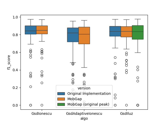
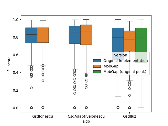
All results across all cohorts#
Note, that the MobGap (original peak) version is a variant of the new GsdIluz algorithm for which we tried
to emulate the original peak detection algorithm as closely as possible.
The regular MobGap version uses a slightly modified peak detection algorithm.
import matplotlib.pyplot as plt
import seaborn as sns

hue_order = ["Original Implementation", "MobGap", "MobGap (original peak)"]

fig, ax = plt.subplots()
sns.boxplot(
    data=results_long,
    x="algo",
    y="f1_score",
    hue="version",
    hue_order=hue_order,
    ax=ax,
)
fig.show()
perf_metrics_all = results_long.pipe(
    multilevel_groupby_apply_merge,
    [
        (
            ["algo", "version"],
            partial(apply_aggregations, aggregations=custom_aggs),
        ),
        (
            ["algo"],
            partial(apply_transformations, transformations=stats_transform),
        ),
    ],
).pipe(format_results)
perf_metrics_all.style.pipe(
    revalidation_table_styles,
    validation_thresholds,
    ["algo"],
)
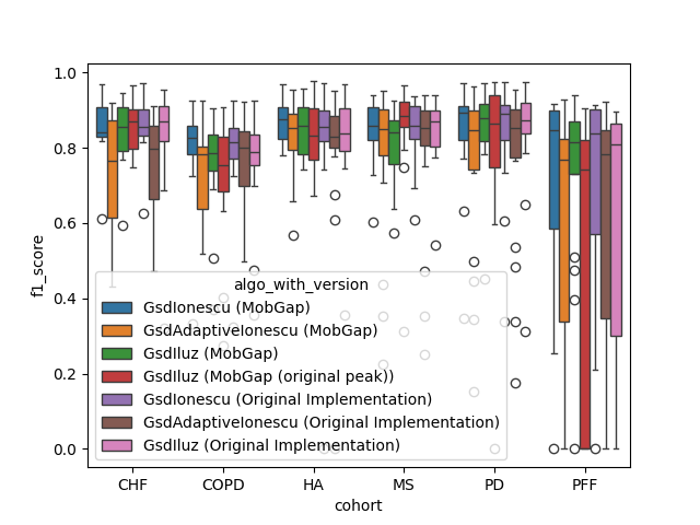
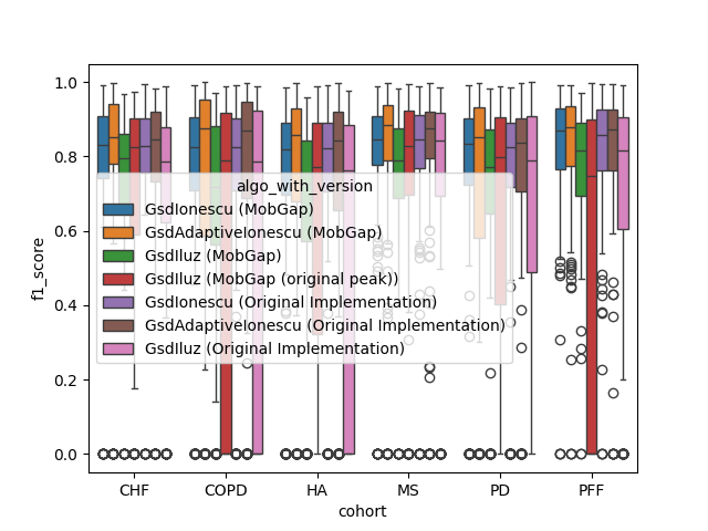
Per Cohort#
While this provides a good overview, it does not fully reflect how these algorithms perform on the different cohorts.
fig, ax = plt.subplots()
sns.boxplot(
    data=results_long, x="cohort", y="f1_score", hue="algo_with_version", ax=ax
)
fig.show()
perf_metrics_per_cohort = (
    results_long.pipe(
        multilevel_groupby_apply_merge,
        [
            (
                ["cohort", "algo", "version"],
                partial(apply_aggregations, aggregations=custom_aggs),
            ),
            (
                ["cohort", "algo"],
                partial(apply_transformations, transformations=stats_transform),
            ),
        ],
    )
    .pipe(format_results)
    .loc[cohort_order]
)
perf_metrics_per_cohort.style.pipe(
    revalidation_table_styles,
    validation_thresholds,
    ["cohort", "algo"],
)
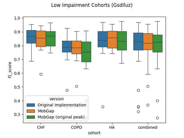
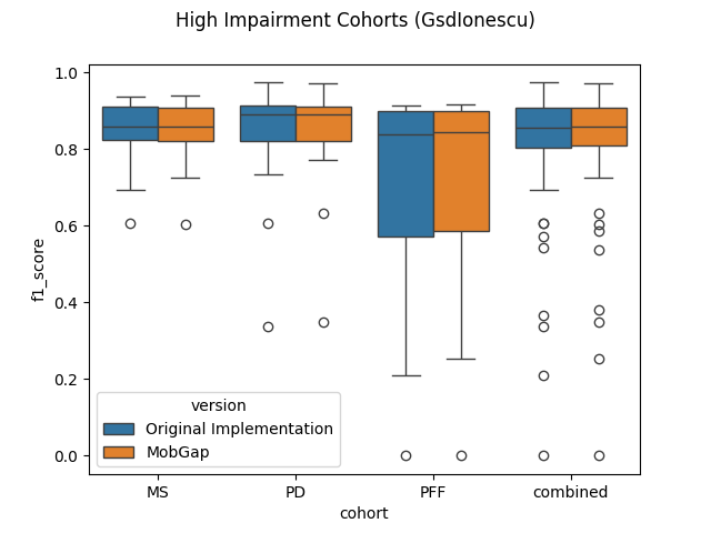
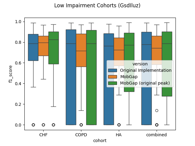
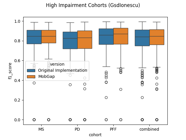
Per relevant cohort#
Overview over all cohorts is good, but this is not how the GSD algorithms are used in our main pipeline.
Here, the HA, CHF, and COPD cohort use the GsdIluz algorithm, while the GsdIonescu algorithm is used for the
MS, PD, PFF cohorts.
Let’s look at the performance of these algorithms on the respective cohorts.
from mobgap.pipeline import MobilisedPipelineHealthy, MobilisedPipelineImpaired

low_impairment_algo = "GsdIluz"
low_impairment_cohorts = list(MobilisedPipelineHealthy().recommended_cohorts)

low_impairment_results = results_long[
    results_long["cohort"].isin(low_impairment_cohorts)
].query("algo == @low_impairment_algo")

fig, ax = plt.subplots()
sns.boxplot(
    data=low_impairment_results,
    x="cohort",
    y="f1_score",
    hue="version",
    hue_order=hue_order,
    ax=ax,
)
sns.boxplot(
    data=low_impairment_results,
    x="_combined",
    y="f1_score",
    hue="version",
    hue_order=hue_order,
    legend=False,
    ax=ax,
)
fig.suptitle(f"Low Impairment Cohorts ({low_impairment_algo})")
fig.show()
perf_metrics_per_cohort.copy().loc[
    pd.IndexSlice[low_impairment_cohorts, low_impairment_algo], :
].reset_index("algo", drop=True).style.pipe(
    revalidation_table_styles,
    validation_thresholds,
    ["cohort"],
)
high_impairment_algo = "GsdIonescu"
high_impairment_cohorts = list(MobilisedPipelineImpaired().recommended_cohorts)

high_impairment_results = results_long[
    results_long["cohort"].isin(high_impairment_cohorts)
].query("algo == @high_impairment_algo")

hue_order = ["Original Implementation", "MobGap"]

fig, ax = plt.subplots()
sns.boxplot(
    data=high_impairment_results,
    x="cohort",
    y="f1_score",
    hue="version",
    hue_order=hue_order,
    ax=ax,
)
sns.boxplot(
    data=high_impairment_results,
    x="_combined",
    y="f1_score",
    hue="version",
    hue_order=hue_order,
    legend=False,
    ax=ax,
)
fig.suptitle(f"High Impairment Cohorts ({high_impairment_algo})")
fig.show()
perf_metrics_per_cohort.copy().loc[
    pd.IndexSlice[high_impairment_cohorts, high_impairment_algo], :
].reset_index("algo", drop=True).style.pipe(
    revalidation_table_styles,
    validation_thresholds,
    ["cohort"],
)
Laboratory Comparison#
Every datapoint below is one trial of a test. Note, that each datapoint is weighted equally in the calculation of the performance metrics. This is a limitation of this simple approach, as the number of strides per trial and the complexity of the context can vary significantly. For a full picture, different groups of tests should be analyzed separately. The approach below should still provide a good overview to compare the algorithms.
All results across all cohorts#
hue_order = ["Original Implementation", "MobGap", "MobGap (original peak)"]

fig, ax = plt.subplots()
sns.boxplot(
    data=lab_results_long,
    x="algo",
    y="f1_score",
    hue="version",
    hue_order=hue_order,
    ax=ax,
)
fig.show()
perf_metrics_all = lab_results_long.pipe(
    multilevel_groupby_apply_merge,
    [
        (
            ["cohort", "algo", "version"],
            partial(apply_aggregations, aggregations=custom_aggs),
        ),
        (
            ["cohort", "algo"],
            partial(apply_transformations, transformations=stats_transform),
        ),
    ],
).pipe(format_results)
perf_metrics_all.style.pipe(
    revalidation_table_styles,
    validation_thresholds,
    ["algo"],
)
Per Cohort#
While this provides a good overview, it does not fully reflect how these algorithms perform on the different cohorts.
fig, ax = plt.subplots()
sns.boxplot(
    data=lab_results_long,
    x="cohort",
    y="f1_score",
    hue="algo_with_version",
    ax=ax,
)
fig.show()
perf_metrics_per_cohort = (
    lab_results_long.pipe(
        multilevel_groupby_apply_merge,
        [
            (
                ["cohort", "algo", "version"],
                partial(apply_aggregations, aggregations=custom_aggs),
            ),
            (
                ["cohort", "algo"],
                partial(apply_transformations, transformations=stats_transform),
            ),
        ],
    )
    .pipe(format_results)
    .loc[cohort_order]
)
perf_metrics_per_cohort.style.pipe(
    revalidation_table_styles,
    validation_thresholds,
    ["cohort", "algo"],
)
Per relevant cohort#
Overview over all cohorts is good, but this is not how the GSD algorithms are used in our main pipeline.
Here, the HA, CHF, and COPD cohort use the GsdIluz algorithm, while the GsdIonescu algorithm is used for the
MS, PD, PFF cohorts.
Let’s look at the performance of these algorithms on the respective cohorts.
low_impairment_results = lab_results_long[
    lab_results_long["cohort"].isin(low_impairment_cohorts)
].query("algo == @low_impairment_algo")

fig, ax = plt.subplots()
sns.boxplot(
    data=low_impairment_results,
    x="cohort",
    y="f1_score",
    hue="version",
    hue_order=hue_order,
    ax=ax,
)
sns.boxplot(
    data=low_impairment_results,
    x="_combined",
    y="f1_score",
    hue="version",
    hue_order=hue_order,
    legend=False,
    ax=ax,
)
fig.suptitle(f"Low Impairment Cohorts ({low_impairment_algo})")
fig.show()
perf_metrics_per_cohort.copy().loc[
    pd.IndexSlice[low_impairment_cohorts, low_impairment_algo], :
].reset_index("algo", drop=True).style.pipe(
    revalidation_table_styles,
    validation_thresholds,
    ["cohort"],
)
high_impairment_results = lab_results_long[
    lab_results_long["cohort"].isin(high_impairment_cohorts)
].query("algo == @high_impairment_algo")

hue_order = ["Original Implementation", "MobGap"]

fig, ax = plt.subplots()
sns.boxplot(
    data=high_impairment_results,
    x="cohort",
    y="f1_score",
    hue="version",
    hue_order=hue_order,
    ax=ax,
)
sns.boxplot(
    data=high_impairment_results,
    x="_combined",
    y="f1_score",
    hue="version",
    hue_order=hue_order,
    legend=False,
    ax=ax,
)
fig.suptitle(f"High Impairment Cohorts ({high_impairment_algo})")
fig.show()
perf_metrics_per_cohort.copy().loc[
    pd.IndexSlice[high_impairment_cohorts, high_impairment_algo], :
].reset_index("algo", drop=True).style.pipe(
    revalidation_table_styles,
    validation_thresholds,
    ["cohort"],
)
Total running time of the script: (0 minutes 24.870 seconds)
Estimated memory usage: 80 MB