Note
Go to the end to download the full example code.
Shin Algo#
This example shows how to use the improved Shin algorithm and some examples on how the results compare to the original matlab implementation.
import pandas as pd
from matplotlib import pyplot as plt
from mobgap.data import LabExampleDataset
from mobgap.initial_contacts import IcdShinImproved
Loading data#
Note
More infos about data loading can be found in the data loading example.
We load example data from the lab dataset together with the INDIP reference system. We will use the INDIP output for initial contacts (“ic”) as ground truth.
from mobgap.utils.conversions import to_body_frame

example_data = LabExampleDataset(
    reference_system="INDIP", reference_para_level="wb"
)

single_test = example_data.get_subset(
    cohort="HA", participant_id="001", test="Test11", trial="Trial1"
)
imu_data = to_body_frame(single_test.data_ss)
reference_wbs = single_test.reference_parameters_.wb_list

sampling_rate_hz = single_test.sampling_rate_hz
ref_ics = single_test.reference_parameters_.ic_list

reference_wbs
Applying the algorithm#
Below we apply the shin algorithm to a lab trial.
We will use the GsIterator to iterate over the gait sequences and apply the algorithm to each wb.
from mobgap.pipeline import GsIterator

iterator = GsIterator()

for (gs, data), result in iterator.iterate(imu_data, reference_wbs):
    result.ic_list = (
        IcdShinImproved()
        .detect(data, sampling_rate_hz=sampling_rate_hz)
        .ic_list_
    )

detected_ics = iterator.results_.ic_list
detected_ics
Matlab Outputs#
To check if the algorithm was implemented correctly, we compare the results to the matlab implementation.
import json

from mobgap import PROJECT_ROOT


def load_matlab_output(datapoint):
    p = datapoint.group_label
    with (
        PROJECT_ROOT
        / f"example_data/original_results/icd_shin_improved/lab/{p.cohort}/{p.participant_id}/SD_Output.json"
    ).open() as f:
        original_results = json.load(f)["SD_Output"][p.time_measure][p.test][
            p.trial
        ]["SU"]["LowerBack"]["SD"]

    if not isinstance(original_results, list):
        original_results = [original_results]

    ics = {}
    for i, gs in enumerate(original_results, start=1):
        ics[i] = pd.DataFrame({"ic": gs["IC"]}).rename_axis(index="step_id")

    return (
        pd.concat(ics, names=["wb_id", ics[1].index.name])
        * datapoint.sampling_rate_hz
    ).astype("int64")


detected_ics_matlab = load_matlab_output(single_test)
detected_ics_matlab
Plotting the results#
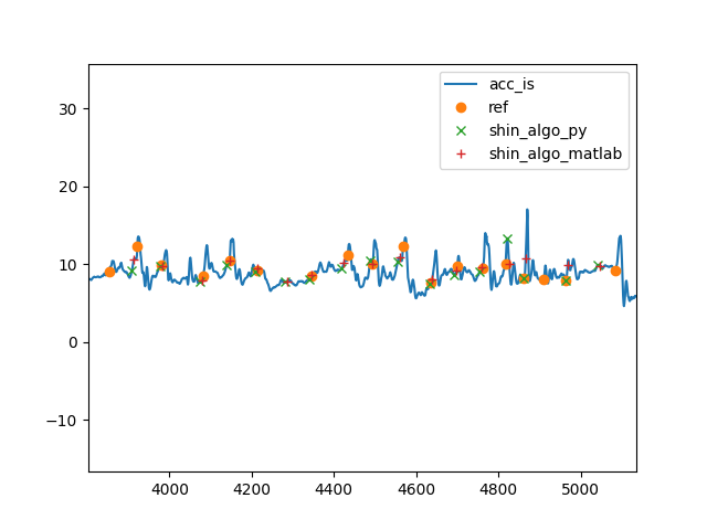
With that we can compare the python, matlab and ground truth results. We zoom in into one of the gait sequences to better see the output.
We can make a couple of main observations:
The python version finds the same ICs as the matlab version, but wil a small shift to the left (around 5-10 samples/50-100 ms). This is likely due to some differences in the downsampling process.
Compared to the ground truth reference, both versions detect the IC too early most of the time.
Both algorithms can not detect the first IC of the gait sequence. However, this is expected, as per definition, this first IC marks the start of the WB in the reference system. Hence, there are no samples before that point the algorithm can use to detect the IC.
imu_data.reset_index(drop=True).plot(y="acc_is")

plt.plot(
    ref_ics["ic"], imu_data["acc_is"].iloc[ref_ics["ic"]], "o", label="ref"
)
plt.plot(
    detected_ics["ic"],
    imu_data["acc_is"].iloc[detected_ics["ic"]],
    "x",
    label="shin_algo_py",
)
plt.plot(
    detected_ics_matlab["ic"],
    imu_data["acc_is"].iloc[detected_ics_matlab["ic"]],
    "+",
    label="shin_algo_matlab",
)
plt.xlim(reference_wbs.iloc[2]["start"] - 50, reference_wbs.iloc[2]["end"] + 50)
plt.legend()
plt.show()
Evaluation of the algorithm against a reference#
To quantify how the Python output compares to the reference labels, we are providing a range of evaluation functions. See the example on ICD evaluation for more details.
Total running time of the script: (0 minutes 1.571 seconds)
Estimated memory usage: 80 MB