Note
Go to the end to download the full example code.
Performance of the laterality classification algorithms on the TVS dataset#
Warning
On this page you will find preliminary results for a standardized revalidation of the pipeline and all of its algorithm. The current state, TECHNICAL EXPERIMENTATION. Don’t use these results or make any assumptions based on them. We will update this page incrementally and provide further information, as soon as the state of any of the validation steps changes.
The following provides an analysis and comparison of the stride length algorithms on the TVS dataset (lab and free-living). We look into the actual performance of the algorithms compared to the reference data.
Compared to the other revalidation scripts, this one does not load the old “matlab” results, as there are no old results. The laterality algorithm by Ulrich et al. was validated independently and was already written in Python. The implemented version follows the old version very closely. The goal of this revalidation, is to validate the re-trained model (with the updated training code) on the TVS dataset. We compare it against the old model and the McCamley algorithm.
Note
If you are interested in how these results are calculated, head over to the processing page.
Below are the list of algorithms that we will compare. Note, that we use the prefix “MobGap” to refer to the newly trained model and “Original Implementation” refers to the models trained as part of previous work. We compare all the available models. For context, the “MS_ALL” models are used by default in the pipelines. For the McCamley algorithm, only a single version exists.
algorithms = {
    "McCamley": ("McCamley", "-"),
    "UllrichOld__ms_all": ("Ullrich - MS-ALL", "Original Implementation"),
    "UllrichOld__ms_ms": ("Ullrich - MS-MS", "Original Implementation"),
    "UllrichNew__ms_all": ("Ullrich - MS-ALL", "MobGap"),
}
The code below loads the data and prepares it for the analysis.
By default, the data will be downloaded from an online repository (and cached locally).
If you want to use a local copy of the data, you can set the MOBGAP_VALIDATION_DATA_PATH environment variable.
and the MOBGAP_VALIDATION_USE_LOCA_DATA to 1.
The file download will print a couple log information, which can usually be ignored.
You can also change the version parameter to load a different version of the data.
from pathlib import Path

import pandas as pd
from mobgap.data.validation_results import ValidationResultLoader
from mobgap.utils.misc import get_env_var


def format_loaded_results(
    values: dict[tuple[str, str], pd.DataFrame],
    index_cols: list[str],
) -> pd.DataFrame:
    formatted = (
        pd.concat(values, names=["algo", "version", *index_cols])
        .reset_index()
        .assign(
            algo_with_version=lambda df: df["algo"]
            + " ("
            + df["version"]
            + ")",
            _combined="combined",
        )
    )
    return formatted


local_data_path = (
    Path(get_env_var("MOBGAP_VALIDATION_DATA_PATH")) / "results"
    if int(get_env_var("MOBGAP_VALIDATION_USE_LOCAL_DATA", 0))
    else None
)
__RESULT_VERSION = "v0.11.0"
loader = ValidationResultLoader(
    "lrc", result_path=local_data_path, version=__RESULT_VERSION
)


free_living_index_cols = [
    "cohort",
    "participant_id",
    "time_measure",
    "recording",
    "recording_name",
    "recording_name_pretty",
]

free_living_results = format_loaded_results(
    {
        v: loader.load_single_results(k, "free_living")
        for k, v in algorithms.items()
    },
    free_living_index_cols,
)

lab_index_cols = [
    "cohort",
    "participant_id",
    "time_measure",
    "test",
    "trial",
    "test_name",
    "test_name_pretty",
]

lab_results = format_loaded_results(
    {
        v: loader.load_single_results(k, "laboratory")
        for k, v in algorithms.items()
    },
    lab_index_cols,
)

cohort_order = ["HA", "CHF", "COPD", "MS", "PD", "PFF"]
  0%|                                              | 0.00/2.44k [00:00<?, ?B/s]
  0%|                                              | 0.00/2.44k [00:00<?, ?B/s]
100%|█████████████████████████████████████| 2.44k/2.44k [00:00<00:00, 12.6MB/s]

  0%|                                              | 0.00/2.43k [00:00<?, ?B/s]
  0%|                                              | 0.00/2.43k [00:00<?, ?B/s]
100%|█████████████████████████████████████| 2.43k/2.43k [00:00<00:00, 17.6MB/s]

  0%|                                              | 0.00/2.44k [00:00<?, ?B/s]
  0%|                                              | 0.00/2.44k [00:00<?, ?B/s]
100%|█████████████████████████████████████| 2.44k/2.44k [00:00<00:00, 18.0MB/s]

  0%|                                              | 0.00/2.41k [00:00<?, ?B/s]
  0%|                                              | 0.00/2.41k [00:00<?, ?B/s]
100%|█████████████████████████████████████| 2.41k/2.41k [00:00<00:00, 16.6MB/s]

  0%|                                              | 0.00/9.56k [00:00<?, ?B/s]
  0%|                                              | 0.00/9.56k [00:00<?, ?B/s]
100%|█████████████████████████████████████| 9.56k/9.56k [00:00<00:00, 63.7MB/s]

  0%|                                              | 0.00/9.68k [00:00<?, ?B/s]
  0%|                                              | 0.00/9.68k [00:00<?, ?B/s]
100%|█████████████████████████████████████| 9.68k/9.68k [00:00<00:00, 67.5MB/s]

  0%|                                              | 0.00/9.65k [00:00<?, ?B/s]
  0%|                                              | 0.00/9.65k [00:00<?, ?B/s]
100%|█████████████████████████████████████| 9.65k/9.65k [00:00<00:00, 68.4MB/s]

  0%|                                              | 0.00/9.05k [00:00<?, ?B/s]
  0%|                                              | 0.00/9.05k [00:00<?, ?B/s]
100%|█████████████████████████████████████| 9.05k/9.05k [00:00<00:00, 63.3MB/s]
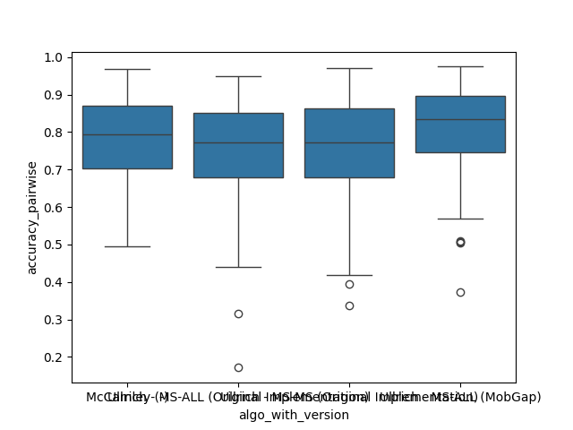
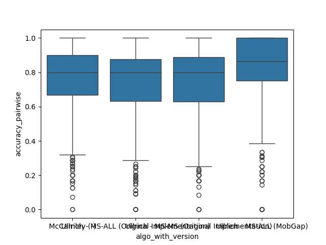
Performance metrics#
Below you can find the setup for all performance metrics that we will calculate. For laterality, this is really simple, as we just calculate the accuracy of the binary classification and the “pariwise accuracy” that checks if consecutive ICs have been assigned either the same or different laterality. High “pairwise accuracy” provides an better indicator if steps and strides would be correctly defined based on the laterality information. This metrics explicitly ignores the actual label of the laterality, as would not impact the main gait metrics, if the laterality is swapped consistently.
from functools import partial

from mobgap.pipeline.evaluation import CustomErrorAggregations as A
from mobgap.utils.df_operations import (
    CustomOperation,
    apply_aggregations,
    apply_transformations,
)
from mobgap.utils.tables import FormatTransformer as F
from mobgap.utils.tables import RevalidationInfo, revalidation_table_styles

custom_aggs = [
    CustomOperation(
        identifier=None,
        function=A.n_datapoints,
        column_name=[("n_datapoints", "all")],
    ),
    ("accuracy", ["mean", A.conf_intervals]),
    ("accuracy_pairwise", ["mean", A.conf_intervals]),
]

format_transforms = [
    CustomOperation(
        identifier=None,
        function=lambda df_: df_[("n_datapoints", "all")].astype(int),
        column_name="n_datapoints",
    ),
    CustomOperation(
        identifier=None,
        function=partial(
            F.value_with_metadata,
            value_col=("mean", "accuracy"),
            other_columns={"range": ("conf_intervals", "accuracy")},
        ),
        column_name="accuracy",
    ),
    CustomOperation(
        identifier=None,
        function=partial(
            F.value_with_metadata,
            value_col=("mean", "accuracy_pairwise"),
            other_columns={"range": ("conf_intervals", "accuracy_pairwise")},
        ),
        column_name="accuracy_pairwise",
    ),
]


final_names = {
    "n_datapoints": "# participants",
    "accuracy": "Accuracy",
    "accuracy_pairwise": "Accuracy IC-pairs",
}

validation_thresholds = {
    "Accuracy": RevalidationInfo(threshold=0.7, higher_is_better=True),
}


def format_tables(df: pd.DataFrame) -> pd.DataFrame:
    return (
        df.pipe(apply_transformations, format_transforms)
        .rename(columns=final_names)
        .loc[:, list(final_names.values())]
    )
Free-Living Comparison#
We focus on the free-living data for the comparison as this is the expected use case for the algorithms.
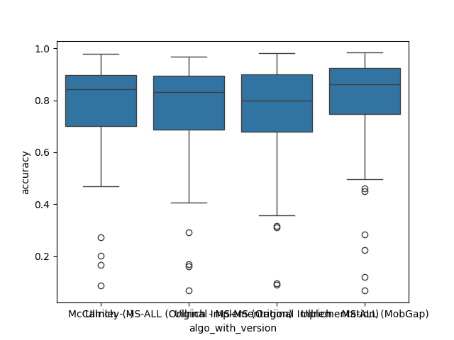
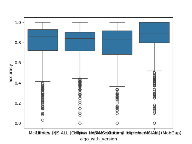
All results across all cohorts#
The results below represent the average performance across all participants independent of the cohort.
import matplotlib.pyplot as plt
import seaborn as sns

fig, ax = plt.subplots()
sns.boxplot(
    data=free_living_results, x="algo_with_version", y="accuracy", ax=ax
)
fig.show()
fig, ax = plt.subplots()
sns.boxplot(
    data=free_living_results,
    x="algo_with_version",
    y="accuracy_pairwise",
    ax=ax,
)
fig.show()

perf_metrics_all = (
    free_living_results.groupby(["algo", "version"])
    .apply(apply_aggregations, custom_aggs, include_groups=False)
    .pipe(format_tables)
)
perf_metrics_all.style.pipe(
    revalidation_table_styles, validation_thresholds, ["algo"]
)
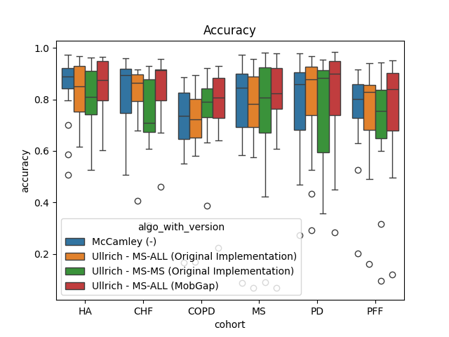
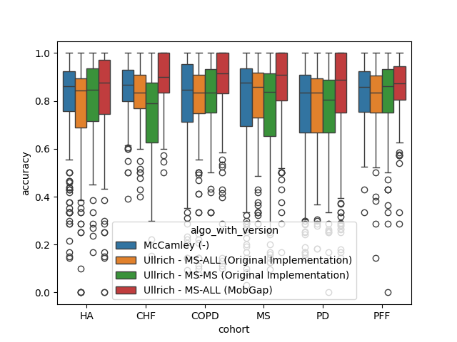
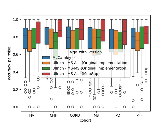
Per Cohort#
The results below represent the average performance across all participants within a cohort.
fig, ax = plt.subplots()
sns.boxplot(
data=free_living_results,
x="cohort",
y="accuracy",
hue="algo_with_version",
order=cohort_order,
ax=ax,
)
ax.set_title("Accuracy")
fig.show()
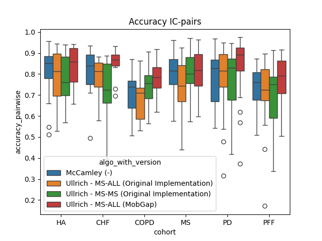
fig, ax = plt.subplots()
sns.boxplot(
data=free_living_results,
x="cohort",
y="accuracy_pairwise",
hue="algo_with_version",
order=cohort_order,
ax=ax,
)
ax.set_title("Accuracy IC-pairs")
fig.show()
perf_metrics_cohort = (
free_living_results.groupby(["cohort", "algo", "version"])
.apply(apply_aggregations, custom_aggs, include_groups=False)
.pipe(format_tables)
.loc[cohort_order]
)
perf_metrics_cohort.style.pipe(
revalidation_table_styles, validation_thresholds, ["cohort", "algo"]
)
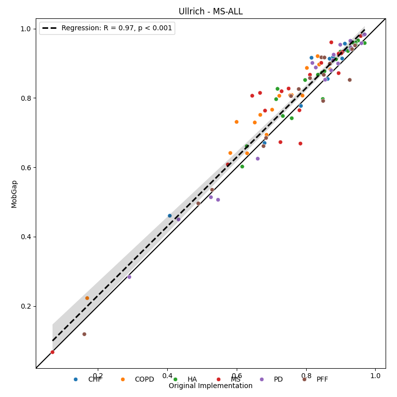
Deep Dive Analysis of Main Algorithms#
Below, we show the direct correlation between the results from the old and the new implementation. Each datapoint represents one participant.
from mobgap.plotting import (
    calc_min_max_with_margin,
    make_square,
    move_legend_outside,
    plot_regline,
)


def compare_scatter_plot(data, name):
    fig, ax = plt.subplots(figsize=(8, 8), constrained_layout=True)
    reformated_data = (
        data.pivot_table(
            values="accuracy",
            index=("cohort", "participant_id"),
            columns="version",
        )
        .reset_index()
        .dropna(how="any")
    )

    min_max = calc_min_max_with_margin(
        reformated_data["Original Implementation"], reformated_data["MobGap"]
    )
    sns.scatterplot(
        reformated_data,
        x="Original Implementation",
        y="MobGap",
        hue="cohort",
        ax=ax,
    )
    plot_regline(
        reformated_data["Original Implementation"],
        reformated_data["MobGap"],
        ax=ax,
    )
    make_square(ax, min_max, draw_diagonal=True)
    move_legend_outside(fig, ax)
    ax.set_title(name)
    ax.set_xlabel("Original Implementation")
    ax.set_ylabel("MobGap")
    plt.tight_layout()
    plt.show()


free_living_results.query("algo == 'Ullrich - MS-ALL'").pipe(
    compare_scatter_plot, "Ullrich - MS-ALL"
)
/home/docs/checkouts/readthedocs.org/user_builds/mobgap/checkouts/v0.11.0/revalidation/laterality/_01_lrc_analysis.py:317: UserWarning: The figure layout has changed to tight
  plt.tight_layout()
Conclusion Free-Living#
It is good to see that the new version of the algorithm performs slightly better than the old version. However, it is unclear, why the new model is different, as we used almost the same pipeline and the same data. The non-ML algo (McCamly) performs suprisingly well, and much better than in the tests we did as part of Mobilise-D. Overall, the performance is not as good as we would like it to be. In particular for a couple of participants, where the performance is as low as 0.1.
Laboratory Comparison#
Every datapoint below is one trial of a test. Note, that each datapoint is weighted equally in the calculation of the performance metrics. This is a limitation of this simple approach, as the number of strides per trial and the complexity of the context can vary significantly. For a full picture, different groups of tests should be analyzed separately. The approach below should still provide a good overview to compare the algorithms.
fig, ax = plt.subplots()
sns.boxplot(data=lab_results, x="algo_with_version", y="accuracy", ax=ax)
fig.show()
fig, ax = plt.subplots()
sns.boxplot(
    data=lab_results, x="algo_with_version", y="accuracy_pairwise", ax=ax
)
fig.show()

perf_metrics_all = (
    lab_results.groupby(["algo", "version"])
    .apply(apply_aggregations, custom_aggs, include_groups=False)
    .pipe(format_tables)
)
perf_metrics_all.style.pipe(
    revalidation_table_styles, validation_thresholds, ["algo"]
)
Per Cohort#
The results below represent the average performance across all trails of all participants within a cohort.
fig, ax = plt.subplots()
sns.boxplot(
    data=lab_results,
    x="cohort",
    y="accuracy",
    hue="algo_with_version",
    order=cohort_order,
    ax=ax,
)
fig.show()
fig, ax = plt.subplots()
sns.boxplot(
    data=lab_results,
    x="cohort",
    y="accuracy_pairwise",
    hue="algo_with_version",
    order=cohort_order,
    ax=ax,
)
fig.show()
perf_metrics_cohort = (
    lab_results.groupby(["cohort", "algo", "version"])
    .apply(apply_aggregations, custom_aggs, include_groups=False)
    .pipe(format_tables)
    .loc[cohort_order]
)
perf_metrics_cohort.style.pipe(
    revalidation_table_styles, validation_thresholds, ["cohort", "algo"]
)
Total running time of the script: (0 minutes 3.741 seconds)
Estimated memory usage: 80 MB