Reorientation Method DM

This example shows how to use the ReorientationMethodDM algorithm to detect and correct persistent IMU misorientation in lower-back-worn devices.

ReorientationMethodDM corrects the most common mounting errors for lower-back-worn, flat rectangular sensors. It assumes that one of the large flat sensor surfaces is mounted against the body and that, under correct mounting, sensor x points along IS, sensor y points along ML, and sensor z points along PA. The method corrects 90 deg and 180 deg mounting rotations, not arbitrary small misalignments.

from __future__ import annotations

Import useful modules and packages

from typing import TYPE_CHECKING

import matplotlib.pyplot as plt
from matplotlib.patches import FancyBboxPatch
from mobgap._gaitmap.utils.rotations import flip_dataset
from mobgap.data import LabExampleDataset
from mobgap.re_orientation import ReorientationMethodDM
from scipy.spatial.transform import Rotation

if TYPE_CHECKING:
    from matplotlib.axes import Axes

Loading some example data

Note

More information about data loading can be found in the data loading example.

We load example data from the lab dataset together with the INDIP reference system.

example_data = LabExampleDataset(
    reference_system="INDIP", reference_para_level="wb"
)

Scope and assumptions

The algorithm groups possible gravity-alignment errors into four orientation families:

• is_up: gravity points up in sensor x (correct orientation).

• is_down: gravity points down in sensor x (180 deg rotation around sensor z).

• ml_up: gravity points up in sensor y (90 deg rotation around sensor z).

• ml_down: gravity points down in sensor y (90 deg rotation around sensor z, then 180 deg rotation around sensor x).

Independently of the gravity direction, the sensor can also be flipped front-to-back around the vertical IS axis. The algorithm estimates this PA direction from the cross-spectral phase between acc_x and acc_z after gravity alignment.

These assumptions are only valid for mostly upright walking bouts. Strongly hunched postures, non-walking activities, or very pathological gait patterns can make the reorientation fail.

Choosing a correction mode

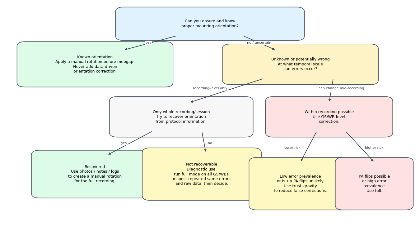
The best reorientation strategy is a good mounting protocol. Knowing the sensor orientation is always better than trying to recover it from the data. If the orientation is known, create and apply the required manual rotation before using mobgap and never add data-driven orientation correction on top.

If orientation errors are still possible, decide at which temporal scale they can occur. If errors can only affect an entire recording or session, try to recover the orientation from protocol information first. For example, operators can take photos of the mounted sensor or record structured mounting notes. If this recovers the orientation, create a manual rotation matrix and apply it to the complete recording before using mobgap.

If a recording-level orientation error cannot be recovered from protocol information, use the reorientation method as a diagnostic tool. Apply it in full mode to all detected gait sequences, or run the full pipeline with reorientation enabled. Then inspect whether an unusually large number of gait sequences report the same misorientation, and inspect the raw data manually. Based on that combined evidence, decide whether to rotate the full recording with a custom orientation matrix.

If orientation errors can occur within a recording, for example because the sensor is loosely attached or participants can remove and reapply it, GS/WB level correction can be appropriate. In this case, choose between the available correction modes:

• trust_gravity first corrects the gravity alignment. If gravity already points up along sensor x (is_up), it trusts that the mounting orientation is correct and skips the PA-direction correction. This intentionally ignores the possible front-to-back flip within the is_up family.

• full applies the PA-direction correction to every walking bout. This can correct the front-to-back flip within is_up, but it also gives the PA-direction classifier more opportunities to introduce false corrections when most walking bouts were already mounted correctly.

The GS/WB-level mode choice is a prevalence problem. If you simulate all supported orientations with equal prevalence, full can look better because every error class is equally likely. In realistic free-living use, however, the identity orientation is often much more common than any single mounting error. By intentionally ignoring one potential error case, we can significantly reduce the likelihood that a correctly oriented sensor is falsely corrected. In the current TVS-based analysis, the rough break-even point between full and trust_gravity is around 33% total misorientation prevalence, or around 7.5% prevalence for the specific is_up front-back flip that trust_gravity intentionally ignores. Treat these values as prevalence guidance, not universal constants.

def _add_decision_box(
    ax: Axes,
    center: tuple[float, float],
    size: tuple[float, float],
    text: str,
    *,
    facecolor: str = "#f7f7f7",
    edgecolor: str = "#4b5563",
) -> None:
    x, y = center
    width, height = size
    box = FancyBboxPatch(
        (x - width / 2, y - height / 2),
        width,
        height,
        boxstyle="round,pad=0.02,rounding_size=0.02",
        facecolor=facecolor,
        edgecolor=edgecolor,
        linewidth=1.4,
        transform=ax.transAxes,
    )
    ax.add_patch(box)
    ax.text(
        x,
        y,
        text,
        ha="center",
        va="center",
        fontsize=9,
        linespacing=1.25,
        transform=ax.transAxes,
    )


def _add_decision_arrow(
    ax: Axes,
    start: tuple[float, float],
    end: tuple[float, float],
    label: str | None = None,
    label_xy: tuple[float, float] | None = None,
) -> None:
    ax.annotate(
        "",
        xy=end,
        xytext=start,
        xycoords=ax.transAxes,
        textcoords=ax.transAxes,
        arrowprops={"arrowstyle": "->", "color": "#374151", "linewidth": 1.4},
    )
    if label and label_xy is not None:
        ax.text(
            *label_xy,
            label,
            ha="center",
            va="center",
            fontsize=8,
            color="#374151",
            bbox={"facecolor": "white", "edgecolor": "none", "pad": 1.5},
            transform=ax.transAxes,
        )


fig, ax = plt.subplots(figsize=(13.5, 8.0))
ax.set_axis_off()

_add_decision_box(
    ax,
    (0.5, 0.92),
    (0.42, 0.1),
    "Can you ensure and know\nproper mounting orientation?",
    facecolor="#e0f2fe",
)
_add_decision_box(
    ax,
    (0.22, 0.75),
    (0.34, 0.15),
    (
        "Known orientation\n"
        "Apply a manual rotation before mobgap.\n"
        "Never add data-driven\n"
        "orientation correction."
    ),
    facecolor="#dcfce7",
)
_add_decision_box(
    ax,
    (0.72, 0.75),
    (0.34, 0.13),
    ("Unknown or potentially wrong\nAt what temporal scale\ncan errors occur?"),
    facecolor="#fef3c7",
)
_add_decision_box(
    ax,
    (0.43, 0.53),
    (0.31, 0.13),
    (
        "Only whole recording/session\n"
        "Try to recover orientation\n"
        "from protocol information."
    ),
)
_add_decision_box(
    ax,
    (0.22, 0.29),
    (0.27, 0.16),
    (
        "Recovered\n"
        "Use photos / notes / logs\n"
        "to create a manual rotation\n"
        "for the full recording."
    ),
    facecolor="#dcfce7",
)
_add_decision_box(
    ax,
    (0.48, 0.29),
    (0.25, 0.18),
    (
        "Not recoverable\n"
        "Diagnostic use:\n"
        "run full mode on all GS/WBs,\n"
        "inspect repeated same errors\n"
        "and raw data, then decide."
    ),
    facecolor="#fef9c3",
)
_add_decision_box(
    ax,
    (0.79, 0.53),
    (0.27, 0.13),
    ("Within recording possible\nUse GS/WB-level\ncorrection."),
    facecolor="#fee2e2",
)
_add_decision_box(
    ax,
    (0.72, 0.25),
    (0.21, 0.18),
    (
        "Low error prevalence\n"
        "or is_up PA flips unlikely\n"
        "Use trust_gravity\n"
        "to reduce false corrections."
    ),
    facecolor="#fef9c3",
)
_add_decision_box(
    ax,
    (0.9, 0.25),
    (0.15, 0.18),
    ("PA flips possible\nor high error\nprevalence\nUse full."),
    facecolor="#fee2e2",
)

_add_decision_arrow(ax, (0.42, 0.87), (0.29, 0.81), "yes", (0.35, 0.84))
_add_decision_arrow(
    ax, (0.58, 0.87), (0.66, 0.81), "no / uncertain", (0.62, 0.84)
)
_add_decision_arrow(
    ax,
    (0.63, 0.69),
    (0.45, 0.59),
    "recording-level only",
    (0.5, 0.65),
)
_add_decision_arrow(
    ax,
    (0.8, 0.69),
    (0.79, 0.59),
    "can change mid-recording",
    (0.82, 0.65),
)
_add_decision_arrow(ax, (0.36, 0.47), (0.25, 0.37), "yes", (0.29, 0.42))
_add_decision_arrow(ax, (0.48, 0.47), (0.49, 0.38), "no", (0.5, 0.42))
_add_decision_arrow(ax, (0.76, 0.47), (0.72, 0.34), "lower risk", (0.7, 0.4))
_add_decision_arrow(ax, (0.83, 0.47), (0.9, 0.34), "higher risk", (0.9, 0.4))

fig.tight_layout()
fig.show()

⤢

Performance on a single lab trial

Below we apply the algorithm to a lab trial, where we extract a single walking bout.

The reorientation algorithm expects sensor-frame input and returns body-frame output.

single_test = example_data.get_subset(
    cohort="HA", participant_id="001", test="Test11", trial="Trial1"
)

reference_wbs = single_test.reference_parameters_.wb_list
sampling_rate_hz = single_test.sampling_rate_hz

# Including only 1 WB as the example
start = reference_wbs.iloc[2]["start"]
end = reference_wbs.iloc[2]["end"]

imu_data = single_test.data.get("LowerBack")
imu_data = imu_data.reset_index(drop=True)

first_wb = imu_data.loc[start:end].copy()

Introducing artificial misorientation

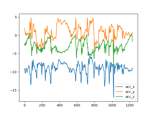
To demonstrate the algorithm, we artificially introduce a misorientation. Below we rotate the sensor frame by 180 degrees around the sensor z-axis (is_down).

first_wb = flip_dataset(first_wb, Rotation.from_euler("z", 180, degrees=True))

print(first_wb)

         acc_x     acc_y     acc_z       gyr_x      gyr_y      gyr_z
3853 -9.063879  1.950392 -2.698835 -103.430341  -4.274265 -41.917592
3854 -9.299348  1.808525 -2.505942 -101.356234  -8.731877 -43.029130
3855 -9.544249  1.662204 -2.348470  -98.319558 -13.819742 -44.106291
3856 -9.610913  1.419515 -2.283629  -96.875704 -17.933579 -43.716680
3857 -9.598021  1.340494 -2.252059  -97.654927 -19.537861 -43.304150
...        ...       ...       ...         ...        ...        ...
5081 -9.108987  0.367603  0.026448  -53.181943  30.550110   1.604282
5082 -9.004980  0.281791 -0.018345  -50.489041  30.160498   0.561499
5083 -8.968239  0.251924 -0.323411  -49.652523  32.039800   0.687549
5084 -9.135023  0.414165 -0.945541  -50.844275  37.070369   0.928192
5085 -9.307359  0.753164 -1.742972  -52.036027  43.602088   1.283425

[1233 rows x 6 columns]

Visualising the misoriented walking bout

We can visualise the walking bout before correction.

fig, ax = plt.subplots()

ax.plot(first_wb["acc_x"].to_numpy(), label="acc_x")
ax.plot(first_wb["acc_y"].to_numpy(), label="acc_y")
ax.plot(first_wb["acc_z"].to_numpy(), label="acc_z")

ax.legend()
fig.show()

⤢

Applying the reorientation algorithm

Below we apply the ReorientationMethodDM algorithm to the misoriented walking bout. We use trust_gravity here to demonstrate the low-prevalence mode. For real data, choose the mode based on the decision tree above.

reoriented = ReorientationMethodDM(
    correction_mode="trust_gravity"
).detect_correct(first_wb, sampling_rate_hz=sampling_rate_hz)

print(f"\nDetected orientation family: {reoriented.result_.family}")
print(f"Correction applied: {reoriented.result_.correction_applied}")
print(f"Correction action: {reoriented.result_.correction_action}")

corrected = reoriented.corrected_data_

Detected orientation family: is_down
Correction applied: True
Correction action: rotated 180 deg around sensor z-axis

Visualising the corrected walking bout

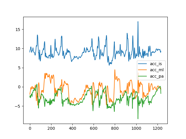
After correction, we can access the corrected data via the corrected_data_ attribute.

fig, ax = plt.subplots()

ax.plot(corrected["acc_is"].to_numpy(), label="acc_is")
ax.plot(corrected["acc_ml"].to_numpy(), label="acc_ml")
ax.plot(corrected["acc_pa"].to_numpy(), label="acc_pa")

ax.legend()
fig.show()

⤢

Estimated memory usage: 86 MB